Create the BEST-COST Multidimensional Deprivation Index (MDI)

This function creates the BEST-COST Multidimensional Deprivation Index (MDI) and checks internal consistency of the single deprivation indicators using Cronbach's coefficient \(\alpha\) and other internal consistency checks

Usage

prepare_mdi(
  geo_id_micro,
  edu,
  unemployed,
  single_parent,
  pop_change,
  no_heating,
  n_quantile,
  verbose = TRUE
)

Arguments

geo_id_micro: Numeric vector or string vector specifying the unique ID codes of each geographic area considered in the assessment (geo_id_micro) Argument must be entered for iterations. See Details for more info.
edu: Numeric vector indicating educational attainment as % of individuals (at the age 18 or older) without a high school diploma (ISCED 0-2) per geo unit
unemployed: Numeric vector containing % of unemployed individuals in the active population (18-65) per geo unit
single_parent: Numeric vector containing single-parent households as % of total households headed by a single parent per geo unit
pop_change: Numeric vector containing population change as % change in population over the previous 5 years (e.g., 2017-2021) per geo unit
no_heating: Numeric vector containing % of households without central heating per geo unit
n_quantile: Integer value specifying the number of quantiles in the analysis.
verbose: Boolean indicating whether function output is printed to console. Default: TRUE.

Value

This function returns a list containing 1) mdi_main (tibble) with the columns (selection);

geo_id_micro containing the numeric geo id's
MDI containing the numeric BEST-COST Multidimensional Deprivation Index values
MDI_index numeric decile based on values in the column MDI
additional columns containing the function input data

2) mdi_detailed (list) with several elements for the internal consistency check of the BEST-COST Multidimensional Deprivation Index.

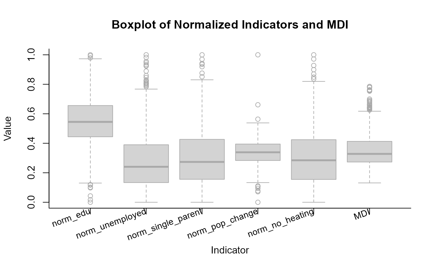
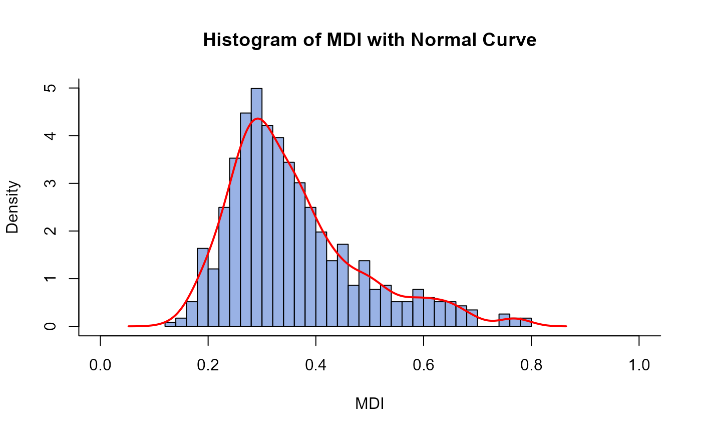
boxplot (language) containing the code to reproduce the boxplot of the single indicators
histogram (language) containing the code to reproduce a histogram of the BEST-COST Multidimensional Deprivation Index (MDI) values with a normal distribution curve
descriptive_statistics (list table of descriptive statistics (mean, SD, min, max) of the normalized input data and the MDI
cronbachs_alpha_value (numeric value See the Details section for the reliability rating this value indicates
pearsons_corr_coeff (numeric vector) Person's correlation coefficient (pairwise-comparisons)

Details

The function outputs Cronbach's \(\alpha\).

\(\alpha \geq\) 0.9: Excellent reliability
0.8 \(\leq \alpha <\) 0.9: Good reliability
0.7 \(\leq \alpha <\) 0.8: Acceptable reliability
0.6 \(\leq \alpha <\) 0.7: Questionable reliability
\(\alpha\) < 0.6: Poor reliability

Data completeness and imputation: ensure the dataset is as complete as possible. You can try to impute missing data:

Time-Based Imputation: Use linear regression based on historical trends if prior years' data is complete.
Indicator-Based Imputation: Use multiple linear regression if the missing indicator correlates strongly with others.

Imputation models should have an R^2 greater than or equal to 0.7. If R^2 lower than 0.7, consider alternative data sources or methods.

See the example below for how to reproduce the boxplots and the histogram after the `prepare_mdi` function call.

Author

Alberto Castro & Axel Luyten

Examples

# Goal: create the BEST-COST Multidimensional Deprivation Index for
# a selection of geographic units

results <- prepare_mdi(
  geo_id_micro = exdat_prepare_mdi$id,
  edu = exdat_prepare_mdi$edu,
  unemployed = exdat_prepare_mdi$unemployed,
  single_parent = exdat_prepare_mdi$single_parent,
  pop_change = exdat_prepare_mdi$pop_change,
  no_heating = exdat_prepare_mdi$no_heating,
  n_quantile = 10,
  verbose = TRUE
)
#> [1] "CRONBACH'S α : 0.746"
#> [1] "Acceptable reliability: 0.7 ≤ α < 0.8"
#> [1] "DESCRIPTIVE STATISTICS"
#>      norm_edu norm_unemployed norm_single_parent norm_pop_change
#> MEAN 0.542    0.289           0.315              0.338          
#> SD   0.171    0.198           0.2                0.09           
#> MIN  0        0               0                  0              
#> MAX  1        1               1                  1              
#>      norm_no_heating MDI      
#> MEAN 0.303           0.357    
#> SD   0.186           0.122    
#> MIN  0               0.1313045
#> MAX  1               0.7855948
#> [1] "PEARSON'S CORRELATION COEFFICIENTS"
#>                     norm_edu norm_unemployed norm_single_parent norm_pop_change
#> norm_edu           1.0000000       0.3773418          0.2526394       0.1494546
#> norm_unemployed    0.3773418       1.0000000          0.9212899       0.2287402
#> norm_single_parent 0.2526394       0.9212899          1.0000000       0.1737842
#> norm_pop_change    0.1494546       0.2287402          0.1737842       1.0000000
#> norm_no_heating    0.5215904       0.3248140          0.3327336       0.2115399
#>                    norm_no_heating
#> norm_edu                 0.5215904
#> norm_unemployed          0.3248140
#> norm_single_parent       0.3327336
#> norm_pop_change          0.2115399
#> norm_no_heating          1.0000000



results$mdi_main |>
  dplyr::select(geo_id_micro, MDI, MDI_index) |>
  dplyr::slice(1:15)
#> # A tibble: 15 × 3
#>    geo_id_micro   MDI MDI_index
#>           <int> <dbl>     <int>
#>  1        11001 0.212         1
#>  2        11002 0.432         8
#>  3        11004 0.185         1
#>  4        11005 0.379         7
#>  5        11007 0.312         5
#>  6        11008 0.257         2
#>  7        11009 0.225         1
#>  8        11013 0.214         1
#>  9        11016 0.266         3
#> 10        11018 0.357         6
#> 11        11021 0.175         1
#> 12        11022 0.211         1
#> 13        11023 0.222         1
#> 14        11024 0.223         1
#> 15        11025 0.248         2

# Reproduce plots after the function call
eval(results$mdi_detailed$boxplot)

eval(results$mdi_detailed$histogram)