Vignette: Intro to healthiar

Hi there!

This vignette will tell you about healthiar and show you how to use healthiar with the help of examples.

NOTE: Before using healthiar, please read carefully the information provided in the readme file or the welcome webpage. By using healthiar, you agree to the terms of use and disclaimer.

About `healthiar`

The healthiar functions allow you to quantify and monetize the health impacts (or burden of disease) attributable to exposure. The main focus of the EU project that initiated the development of healthiar (BEST-COST) has been two environmental exposures: air pollution and noise. However, healthiar could be used for other exposures such as green spaces, chemicals, physical activity…

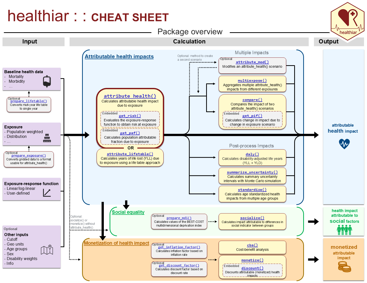
See below a an overview of the healthiar, which is the first page of the cheat sheet. The whole list of functions included in healthiar is linked there and available in the reference.

Figure: Overview of healthiar

Input & output data

Input

You can enter data in healthiar functions using: - hard coded values or - columns inside pre-loaded data frames or tibbles.

Let’s see some examples calling the most important function in healthiar: attribute_health().

Hard coded vs. columns

Hard coded

Depending on the function argument, you will need to enter numeric or character values.

results_pm_copd <- attribute_health(
  exp_central = 8.85, 
  rr_central = 1.369, 
  rr_increment = 10,  
  erf_shape = "log_linear",
  cutoff_central = 5,
  bhd_central = 30747 
)

Columns

healthiar comes with some example data that start with exdat_ that allow you to test functions. Some of these example data will be used in some examples in this vignette.

Now let’s attribute_health() with input data from the healthiar example data. Note that you can easily provide input data to the function argument using the $ operator.

results_pm_copd <- attribute_health(
  erf_shape = "log_linear",
  rr_central = exdat_pm$relative_risk, 
  rr_increment = 10, 
  exp_central = exdat_pm$mean_concentration,
  cutoff_central = exdat_pm$cut_off_value,
  bhd_central = exdat_pm$incidence
)

Tidy data

Be aware that healthiar functions are easier to use if your data is prepared in a tidy format, i.e.:

Each variable is a column; each column is a variable.
Each observation is a row; each row is an observation.
Each value is a cell; each cell is a single value.

To know more about the concept of tidy format, see the article by (Wickham 2014).

For example, in attribute health() the length of the input vectors to be entered in the arguments must be either 1 or the result of the combinations of the different values of:

geo_id_micro
exp_...
sex
age
(info for further sub-group analysis)

Output

Structure

The output of the healthiarfunction attribute_health() and attribute_lifetable consists of two lists (“folders”):

health_main contains the main results
health_detailed contained detailed results and additional info about the assessment.

In other healthiar functions you can find a similar output structure but using different prefixes. E.g., social_in socialize() and monetization_in monetitize().

Access

A similar structure can be found in other large functions in helathiar, e.g., attribute_lifetable(), compare(), socialize() or monetize(). In some functions, different elements are available in the output. For instance, attribute_lifetable() creates additional output that is specific to life table calculations.

There exist different, equivalent ways of accessing the output:

With $ operator: results_pm_copd$health_main$impact_rounded (as in the example above)
By mouse: go to the Environment tab in RStudio and click on the variable you want to inspect, and then open the health_main results table
With [[]] operator results_pm_copd[["health_main"]]
With pluck() & pull(): use the purrr::pluck function to select a list and then the dplyr::pull function extract values from a specified column, e.g. results_pm_copd |> purrr::pluck("health_main") |> dplyr::pull("impact_rounded")

Function examples

The descriptions of the healthiar functions provide examples that you can execute (with healthiar loaded) by running example("function_name"), e.g. example("attribute_health"). In the sections below in this vignette, you find additional examples and more detailed explanations.

Relative risk

Goal

E.g., to quantify the COPD cases attributable to PM2.5 (air pollution) exposure in a country.

Methodology

The comparative risk assessment approach (C. J. Murray et al. 2003) is applied obtaining the population attributable fraction (percent of cases that are attributable to the exposure) based on the relative risk. The exposure scenario is compared with a counter-factual scenario.

This approach has been extensive documented and applied (e.g., WHO 2003; Steenland and Armstrong 2006; Soares et al. 2022; Pozzer et al. 2023; GBD 2019 Risk Factors Collaborators 2020; Lehtomäki et al. 2025).

Figure: Relative risk approach

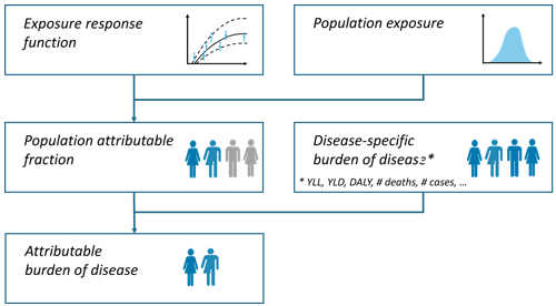
Population attributable fraction

General integral form for the population attributable fraction (PAF):

$PAF = \frac{\int rr\_at\_exp(x) \times PE(x)dx - 1}{\int rr\_at\_exp(x) \times pop\_exp(x)dx}$

Where:

$x$ = exposure level
$PE(x)$ = population distribution of exposure
$rr\_at\exp(x)$ = relative risk at exposure level compared to reference

Simplified for categorical exposure distribution

If exposure is categorical, the integrals are converted to sums:

$PAF = \frac{\sum rr\_at\_exp_i \times PE_i - 1}{\sum rr\_at\_exp_i \times PE_i}$

Alternatively, an equivalent form is:

$PAF = \frac{\sum PE_i \times (rr\_at\_exp_i - 1)}{\sum PE_i\times (rr\_at\_exp_i - 1) + 1}$

Simplified for single exposure value

If there is one single single exposure value, corresponding to the population weighted mean concentration, the equation can be simplified as follows:

$PAF = \frac{rr\_at\_exp - 1}{rr\_at\_exp }$ #### Scaling relative risk How to get this relative risk at exposure level (rr_at_exp)? This is normally different to the relative risk published in the epidemiological literature (rr) together with the (concentration/dose) increment that corresponds to this relative risk. The equations used for scaling relative risk depend on the chosen exposure-response function shapes:

linear [Lehtomaki_2025_eh] $RRexp = 1 + \frac{rr - 1}{increment} \times (exp - cutoff)$
log-linear (Lehtomäki et al. 2025) $RRexp = e^{\frac{\log(rr)}{increment} \times (exp - cutoff)}$
log-log (Lehtomäki et al. 2025) $RRexp = \left( \frac{exp + 1}{cutoff + 1} \right)^{\frac{\log(rr)}{\log(increment + cutoff + 1) - \log(cutoff + 1)}}$
linear-log (Pozzer et al. 2023) $RRexp = 1 + \frac{\log(rr - 1)}{\log(increment + cutoff + 1) - \log(cutoff + 1)} \times \frac{\log(exp + 1)}{\log(cutoff + 1)}$

The relative risk at exposure level (rr_at_exp) and is part of the output of attribute_health() and attribute_lifetable(). rr_at_exp can also be calculated using get_risk().

For conversion of hazard ratios and/or odds ratios to relative risks refer to (VanderWeele 2019) and/or use the conversion tools developed by the Teaching group in EBM in 2022 for hazard ratios (https://ebm-helper.cn/en/Conv/HR_RR.html) and/or odds ratios (https://ebm-helper.cn/en/Conv/OR_RR.html).

Function call

results_pm_copd <- attribute_health(
  approach_risk = "relative_risk", # If you do not call this argument, "relative_risk" will be assigned by default.
  erf_shape = "log_linear",
  rr_central = exdat_pm$relative_risk, 
  rr_increment = 10, 
  exp_central = exdat_pm$mean_concentration,
  cutoff_central = exdat_pm$cut_off_value,
  bhd_central = exdat_pm$incidence
)

Main results

results_pm_copd$health_main
#> # A tibble: 1 × 24
#>   geo_id_micro erf_ci  exp_ci  bhd_ci  cutoff_ci exp_category sex   age_group
#>   <chr>        <chr>   <chr>   <chr>   <chr>            <int> <chr> <chr>    
#> 1 a            central central central central              1 all   all      
#> # ℹ 16 more variables: impact <dbl>, impact_rounded <dbl>, approach_risk <chr>,
#> #   rr_increment <dbl>, erf_shape <chr>, prop_pop_exp <dbl>, exp_length <int>,
#> #   exp_type <chr>, exp <dbl>, bhd <dbl>, cutoff <dbl>, rr <dbl>,
#> #   is_lifetable <lgl>, pop_fraction_type <chr>, rr_at_exp <dbl>,
#> #   pop_fraction <dbl>

It is a table of the format tibble of 3 rows and 23 columns. Be aware that this main output contains input data, some intermediate steps and the final results in different formats.

Let’s zoom in on some relevant aspects.

results_pm_copd$health_main |> 
  dplyr::select(exp, bhd, rr, erf_ci, pop_fraction, impact_rounded) |> 
  knitr::kable() # For formatting reasons only: prints tibble in nice layout

exp	bhd	rr	erf_ci	pop_fraction	impact_rounded
8.85	30747	1.369	central	0.1138961	3502

Interpretation: this table shows us that exposure was 8.85 $\mu g/m^3$ , the baseline health data (bhd_central) was 30747 (COPD incidence in this instance). The 1st row further shows that the impact attributable to this exposure using the central relative risk (rr_central) estimate of 1.369 is 3502 COPD cases, or ~11% of all baseline cases.

Some of the most results columns include:

impact_rounded rounded attributable health impact/burden
impact raw impact/burden
pop_fraction population attributable fraction (PAF) or population impact fraction (PIF)

Absolute risk

Goal

E.g., to quantify the number incidence cases of high annoyance attributable to (road traffic) noise exposure.

Methodology

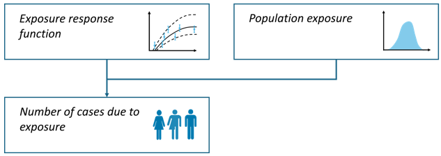
In the absolute risk calculation pathway, estimates are based on the size and distribution of the exposed population, rather than on baseline health data, as is the case in the relative risk pathway (WHO 2011).

Figure: Absolute risk approach

$N = \sum AR_i \times PE_i$

Where:

$N$ = attributed cases
$AR_i$ = absolute risk at category $i$
$PE_i$ = absolute population exposed at category $i$

Function call

results_noise_ha <- attribute_health(
  approach_risk = "absolute_risk", # default is "relative_risk"
  exp_central = c(57.5, 62.5, 67.5, 72.5, 77.5), # mean of the exposure categories
  pop_exp = c(387500, 286000, 191800, 72200, 7700), # population exposed per exposure category
  erf_eq_central = "78.9270-3.1162*c+0.0342*c^2" # exposure-response function
)

The erf_eq_central argument can digest other types of functions (see section on user-defined ERF).

Main results

erf_eq	erf_ci	impact_rounded
78.9270-3.1162c+0.0342c^2	central	174232

Results per noise exposure band

results_noise_ha$health_detailed$results_raw

exp_category	exp	pop_exp	impact
1	57.5	387500	49674.594
2	62.5	286000	50788.595
3	67.5	191800	46813.105
4	72.5	72200	23657.232
5	77.5	7700	3298.314

Remember, that if the equation of the exposure-response function (erf_eq_...) requires taking a maximum in a vectorised context, pmax() must be used instead of max(). pmax() should be used whenever an element-wise maximum is required (the output will be a vector), while max() returns a single global maximum for the entire vector. For example:

erf_eq_central <- 
  "exp(0.2969*log((pmax(0,c-2.4)/1.9+1))/(1+exp(-(pmax(0,c-2.4)-12)/40.2)))"

One exposure category

Alternatively, it’s also possible to only assess the absolute risk impacts for one exposure category (e.g., a single noise exposure band).

results_noise_ha <- attribute_health(
  approach_risk = "absolute_risk",
  exp_central = 57.5,
  pop_exp = 387500,
  erf_eq_central = "78.9270-3.1162*c+0.0342*c^2"
)

exp_category	impact
1	49674.59

Multiple geographic units

using relative risk

Goal

E.g., to quantify the disease cases attributable to PM2.5 exposure in multiple cities using one single command.

Function call

Enter unique ID’s as a vector (numeric or character) to the geo_id_micro argument (e.g., municipality names or province abbreviations)
Optional: aggregate unit-specific results by providing higher-level ID’s (e.g., region names or country abbreviations) as a vector (numeric or character) to the geo_id_macro argument

Input to the other function arguments is specified as usual, either as a vector or a single values (which will be recycled to match the length of the other input vectors).

results_iteration <- attribute_health(
    # Names of Swiss cantons
    geo_id_micro = c("Zurich", "Basel", "Geneva", "Ticino", "Jura"),
    # Names of languages spoken in the selected Swiss cantons
    geo_id_macro = c("German","German","French","Italian","French"),
    rr_central = 1.369,
    rr_increment = 10, 
    cutoff_central = 5,
    erf_shape = "log_linear",
    exp_central = c(11, 11, 10, 8, 7),
    bhd_central = c(4000, 2500, 3000, 1500, 500)
)

In this example we want to aggregate the lower-level geographic units (municipalities) by the higher-level language region ("German", "French", "Italian").

Main results

The main output contains aggregated results

geo_id_macro	impact_rounded	erf_ci	exp_ci	bhd_ci
German	1116	central	central	central
French	466	central	central	central
Italian	135	central	central	central

In this case health_main contains the cumulative / summed number of stroke cases attributable to PM2.5 exposure in the 5 geo units, which is 1717 (using a relative risk of 1.369).

Detailed results

The geo unit-specific information and results are stored under health_detailed>results_raw .

geo_id_micro	impact_rounded	geo_id_macro
Zurich	687	German
Basel	429	German
Geneva	436	French
Ticino	135	Italian
Jura	30	French

health_detailed also contains impacts obtained through all combinations of input data central, lower and upper estimates (as usual), besides the results per geo unit (not shown above).

using absolute risk

Goal

E.g., to quantify high annoyance cases attributable to noise exposure in rural and urban areas.

Function call

data <- exdat_noise |> 
  ## Filter for urban and rural regions
  dplyr::filter(region == "urban" | region == "rural")

results_iteration_ar <- attribute_health( 
    # Both the rural and urban areas belong to the higher-level "total" region
    geo_id_macro = "total",
    geo_id_micro = data$region,
    approach_risk = "absolute_risk",
    exp_central = data$exposure_mean,
    pop_exp = data$exposed,
    erf_eq_central = "78.9270-3.1162*c+0.0342*c^2"
)

NOTE: the length of the input vectors fed to geo_id_micro, exp_central, pop_exp must match and must be

(number of geo units) x (number of exposure categories) = 2 x 5 = 10,

because we have 2 geo units ("rural" and "urban") and 5 exposure categories.

Main results

health_main contains the aggregated results (i.e. sum of impacts in rural and urban areas).

geo_id_macro	impact_rounded	erf_ci	exp_ci
total	174232	central	central

Detailed results

Impact by geo unit, in this case impact in the rural and in the urban area.

geo_id_micro	geo_id_macro	impact
urban	total	150904.00
rural	total	23327.84

Uncertainty

Confidence interval

Goal

E.g., to quantify the COPD cases attributable to PM2.5 exposure taking into account uncertainty (lower and upper bound of confidence interval) in several input arguments: relative risk, exposure and baseline health data.

Function call

results_pm_copd <- attribute_health(
    erf_shape = "log_linear",
    rr_central = 1.369, 
    rr_lower = 1.124, # lower 95% confidence interval (CI) bound of RR
    rr_upper = 1.664, # upper 95% CI bound of RR
    rr_increment = 10, 
    exp_central = 8.85, 
    exp_lower = 8, # lower 95% CI bound of exposure
    exp_upper = 10, # upper 95% CI bound of exposure
    cutoff_central = 5,
    bhd_central = 30747, 
    bhd_lower = 28000, # lower 95% confidence interval estimate of BHD
    bhd_upper = 32000 # upper 95% confidence interval estimate of BHD
)

Detailed results

Let’s inspect the detailed results:

erf_ci	exp_ci	bhd_ci	impact_rounded
central	central	central	3502
lower	central	central	1353
upper	central	central	5474
central	central	lower	3189
lower	central	lower	1232
upper	central	lower	4985
central	central	upper	3645
lower	central	upper	1408
upper	central	upper	5697

Each row contains the estimated attributable cases (impact_rounded) obtained by the input data specified in the columns ending in “_ci” and the other calculation pathway specifications in that row (not shown).

The 1st contains the estimated attributable impact when using the central estimates of relative risk, exposure and baseline health data.
The 2nd row shows the impact when using the central estimates of the relative risk, exposure in combination with the lower estimate of the baseline health data.
…

NOTE: only 9 of the 27 possible combinations are displayed due to space constraints.

NOTE: only a selection of columns are shown.

Monte Carlo simulation

Goal

E.g., to summarize uncertainty of attributable health impacts (i.e. to get a single confidence interval instead of many combinations) by using a Monte Carlo simulation.

Methodology

General concepts

A Monte Carlo simulation is a statistical method that generates repeated random sampling [Robert and Casella (2004); Rubinstein and Kroese (2016). In healthiar, you can use the function summarize_uncertainty() to simulate values in the arguments with uncertainty and estimate a single confidence interval in the results.

For each entered input argument that includes a (95%) confidence interval (i.e. _lower and _upper bound value) a distribution is fitted (see distributions below). The median of the simulated attributable impacts is reported as the central estimate. The 2.5th and 97.5th percentiles of these simulated impacts define the lower and upper bounds of the 95% summary uncertainty interval. Aggregated central, lower and upper estimates are obtained by summing the corresponding values of each lower level unit.

Distributions used for simulation

summarize_uncertainty() assumes the following shapes of the distributions in the simulations:

Relative risk: The values are simulated based on an optimized gamma distribution, which fits well as relative risks are positive and their distributions are usually right-skewed. The gamma distribution is parametrized such that its mean is equal to the central relative risk estimate (rate= shape/rr_central). The shape parameter is then optimized using stats::optimize() to match the inputed 95% confidence interval bounds, with stats::qgamma() used to evaluate candidate distributions. Finally, n_sim relative risk values are simulated using stats::rgamma().
Exposure, cutoff, baseline health data and duration: The values are simulated based on a normal distribution using stats::rnorm() with mean = exp_central, mean = cutoff_central, mean = bhd_central or mean = duration_central and a standard deviation based on corresponding lower and upper 95% exposure confidence interval values. The standard deviation is calculated as $(upper-lower)/(2*1.96)$ , since for a normal distribution the 95% CI spans approximately two standard deviations on either side of the mean.
Disability weights: The values are simulated based on a beta distribution, as both the disability weights and the beta distribution are bounded by 0 and 1. The beta distribution best fitting the inputted central disability weight estimate and corresponding lower and upper 95% confidence interval values is fitted using stats::qbeta() (the best fitting distribution parameters shape1 and shape2 are determined using stats::optimize()). For this purpose, we partly adapted the R function prevalence::beta_expert with permission of one of the authors (Devleesschauwer et al. 2022). Finally, n_sim disability weight values are simulated using stats::rbeta().

For stability of the 95% confidence interval, a large number of simulations (e.g., 10,000) is recommended in practice. The example below uses n_sim = 100 for brevity.

Function call

results_pm_copd_summarized <- 
  summarize_uncertainty(
    output_attribute = results_pm_copd,
    n_sim = 100
)

Main results

The outcome of the Monte Carlo analysis is added to the variable entered as the results argument, which is results_pm_copd in our case.

Two lists (“folders”) are added:

uncertainty_main contains the central estimate and the corresponding 95% confidence intervals obtained through the Monte Carlo assessment and
uncertainty_detailed contains all n_sim simulations of the Monte Carlo assessment.

geo_id_micro	impact_ci	impact	impact_rounded
a	central_estimate	3654.885	3655
a	lower_estimate	1589.442	1589
a	upper_estimate	5600.248	5600

Detailed results

The folder uncertainty_detailed contains all single simulations. Let’s look at the impact of the first 10 simulations.

The columns erf_ci, exp_ci, bhd_ci, and cutoff_ci indicate the source of uncertainty component used for that simulation (in the first 10 simulations, all use central estimates).

geo_id_micro	erf_ci	exp_ci	bhd_ci	cutoff_ci	exp_category	sex	age_group	sim_id	impact	impact_rounded	approach_risk	rr_increment	erf_shape	prop_pop_exp	exp_length	exp_type	cutoff	is_lifetable	geo_id_number	rr	exp	bhd	pop_fraction_type	rr_at_exp	pop_fraction
a	central	central	central	central	1	all	all	1	2629.951	2630	relative_risk	10	log_linear	1	1	population_weighted_mean	5	FALSE	1	1.276850	8.740519	30103.82	paf	1.095725	0.0873627
a	central	central	central	central	1	all	all	2	4628.066	4628	relative_risk	10	log_linear	1	1	population_weighted_mean	5	FALSE	1	1.551852	8.758388	30399.07	paf	1.179584	0.1522437
a	central	central	central	central	1	all	all	3	4493.994	4494	relative_risk	10	log_linear	1	1	population_weighted_mean	5	FALSE	1	1.543406	8.798881	29566.80	paf	1.179238	0.1519946
a	central	central	central	central	1	all	all	4	4474.906	4475	relative_risk	10	log_linear	1	1	population_weighted_mean	5	FALSE	1	1.419867	9.213612	32586.97	paf	1.159181	0.1373219
a	central	central	central	central	1	all	all	5	1650.331	1650	relative_risk	10	log_linear	1	1	population_weighted_mean	5	FALSE	1	1.157613	8.812466	30409.10	paf	1.057385	0.0542710
a	central	central	central	central	1	all	all	6	3728.251	3728	relative_risk	10	log_linear	1	1	population_weighted_mean	5	FALSE	1	1.430150	8.830799	29108.69	paf	1.146895	0.1280803
a	central	central	central	central	1	all	all	7	3879.688	3880	relative_risk	10	log_linear	1	1	population_weighted_mean	5	FALSE	1	1.465879	8.502208	30948.22	paf	1.143328	0.1253606
a	central	central	central	central	1	all	all	8	3917.858	3918	relative_risk	10	log_linear	1	1	population_weighted_mean	5	FALSE	1	1.442681	8.684553	31015.55	paf	1.144583	0.1263191
a	central	central	central	central	1	all	all	9	3038.873	3039	relative_risk	10	log_linear	1	1	population_weighted_mean	5	FALSE	1	1.320146	8.880695	29741.04	paf	1.113806	0.1021778
a	central	central	central	central	1	all	all	10	2145.128	2145	relative_risk	10	log_linear	1	1	population_weighted_mean	5	FALSE	1	1.253879	8.549538	27799.07	paf	1.083618	0.0771655

User-defined ERF

Goal

E.g., to quantify COPD cases attributable to air pollution exposure by applying a user-defined exposure-response function (ERF), such as the MR-BRT curves from Global Burden of Disease study.

Function call

In this case, the function arguments erf_eq_... require a function as input, so we use an auxiliary function (splinefun()) to transform the points on the ERF into type function.

results_pm_copd_mr_brt <- attribute_health(
  exp_central = 8.85,
  bhd_central = 30747,
  cutoff_central = 0,
  # Specify the function based on x-y point pairs that lie on the ERF
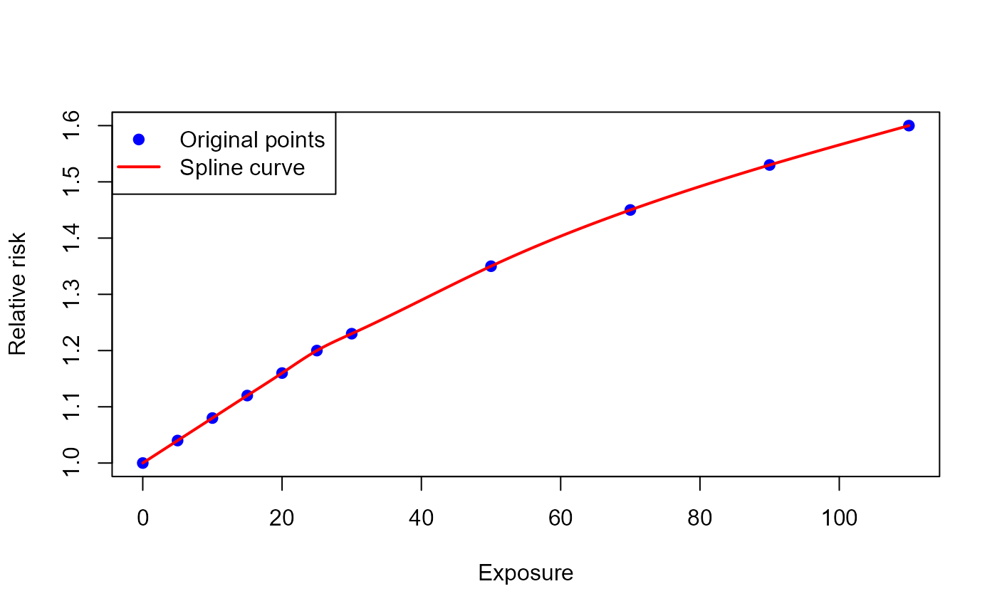
  erf_eq_central = splinefun(
    x = c(0, 5, 10, 15, 20, 25, 30, 50, 70, 90, 110),
    y = c(1.00, 1.04, 1.08, 1.12, 1.16, 1.20, 1.23, 1.35, 1.45, 1.53, 1.60),
    method = "natural")
)

The ERF curve created looks as follows

ERF curve

Alternatively, other functions (e.g. approxfun()) can be used to create the ERF

Sub-group analysis

by age group

Goal

E.g., to quantify health impacts attributable to air pollution in a country by age group.

Function call

To obtain age-group-specific results, the baseline health data (and possibly exposure) must be available by age group.

If the age argument was specified, age-group-specific results are available under health_detailed in the sub-folder results_by_age_group.

results_age_group <- attribute_health(
        approach_risk = "relative_risk",
        age = c("below_65", "65_plus"),
        exp_central = c(8, 7),
        cutoff_central = c(5, 5),
        bhd_central = c(1000, 5000),
        rr_central = 1.06,
        rr_increment = 10,
        erf_shape = "log_linear"
      )

Results by age group

results_age_group$health_detailed$results_by_age_group |> 
  dplyr::select(age_group, impact_rounded, exp, bhd) |> 
  knitr::kable()

age_group	impact_rounded	exp	bhd
below_65	17	8	1000
65_plus	58	7	5000

by sex

Goal

E.g., to quantify health impacts attributable to air pollution in a country by sex.

Function call

The baseline health data (and possibly exposure) must be entered by sex.

results_sex <- attribute_health(
        approach_risk = "relative_risk",
        sex = c("female", "male"),
        exp_central = c(8, 8),
        cutoff_central = c(5, 5),
        bhd_central = c(1000, 1100),
        rr_central = 1.06,
        rr_increment = 10,
        erf_shape = "log_linear"
      )

Results by sex

If the sex argument was specified, sex-specific results are available under health_detailed in the sub-folder results_by_sex.

results_sex$health_detailed$results_by_sex |> 
  dplyr::select(sex, impact_rounded, exp, bhd) |> 
  knitr::kable()

sex	impact_rounded	exp	bhd
female	17	8	1000
male	19	8	1100

by other sub-groups

Goal

E.g., to quantify attributable health impacts stratified by a sub-group different to age and sex, e.g., education level.

Function call

A single vector (or a data frame / tibble with multiple columns) to group the results by can be entered to the info argument. In this example, this will be information about the education level.

In a second step one can group the results based on one or more columns and so summarize the results by the preferred sub-groups.

output_attribute <- healthiar::attribute_health(
    rr_central = 1.063,
    rr_increment = 10,
    erf_shape = "log_linear",
    cutoff_central =  0,
    exp_central = c(6, 7, 8,
                    7, 8, 9,
                    8, 9, 10,
                    9, 10, 11),
    bhd_central = c(600, 700, 800,
                    700, 800, 900,
                    800, 900, 1000,
                    900, 1000, 1100),
    geo_id_micro = rep(c("a", "b", "c", "d"), each = 3),
    info = data.frame(
      education = rep(c("secondary", "bachelor", "master"), times = 4)) # education level
  )

Results by other sub-group

output_stratified <- output_attribute$health_detailed$results_raw |>
      dplyr::group_by(info_column_1) |>
      dplyr::summarize(mean_impact = mean(impact))|>
      dplyr::pull(mean_impact) |>
      print()
#> [1] 43.72087 54.26844 34.30332

by age, sex and other sub-groups

Goal

E.g., to quantify attributable health impacts stratified by age, sex and additional sub-group e.g. education level.

Function call

output_attribute <- healthiar::attribute_health(
    rr_central = 1.063,
    rr_increment = 10,
    erf_shape = "log_linear",
    cutoff_central =  0,
    age_group = base::rep(c("50_and_younger", "50_plus"), each = 4, times= 2),
    sex = base::rep(c("female", "male"), each = 2, times = 4),
    exp_central = c(6, 7, 8, 7, 8, 9, 8, 9,
                    10, 9, 10, 11, 10, 11, 12, 13),
    bhd_central = c(600, 700, 800, 700, 800, 900, 800, 900,
                    1000, 900, 1000, 1100, 1000, 1100, 1200, 1000),
    geo_id_micro = base::rep(c("a", "b"), each = 8),
    info = base::data.frame(
      education = base::rep(c("without_master", "with_master"), times = 8)) # education level
  )

Results by all sub-groups

output_stratified <- output_attribute$health_detailed$results_raw |>
      dplyr::group_by(info_column_1) |>
      dplyr::summarize(mean_impact = mean(impact))|>
      dplyr::pull(mean_impact) |>
      print()
#> [1] 52.80090 49.83826

YLL & deaths with life table

YLL

Goal

E.g., to quantify the years of life lost (YLL) due to deaths from COPD attributable to PM2.5 exposure during one year.

Methodology

Data preparation

The life table approach to obtain YLL and deaths requires population and baseline mortality data to be stratified by one year age groups. However, in some cases these data are only available for larger age groups (e.g., 5-year data: 0-4 years old, 5-9 years old, …). What to do?

If your population and mortality data are not available by one-year age group, your data must be prepared by interpolating values. The healthiar function prepare_lifetable() makes this conversion using the same approach as the WHO tool AirQ+ (WHO 2020).
If your population and death data are stratified by one-year age group, you are lucky, you can ignore this initial step.

General concept

The life table methodology of attribute_lifetable() follows that of the WHO tool AirQ+ (WHO 2020), which is described in more detail by B. G. Miller and Hurley (2003).

In short, two scenarios are compared:

a scenario with the exposure level specified in the function (“exposed scenario”) and
a scenario with no exposure (“unexposed scenario”).

First, the entry and mid-year populations of the (first) year of analysis in the unexposed scenario is determined using modified survival probabilities. Second, age-specific population projections using scenario-specific survival probabilities are done for both scenarios. Third, by subtracting the populations in the unexposed scenario from the populations in the exposed scenario the premature deaths/years of life lost attributable to the exposure are determined.

An expansive life table case study for is available in a report of Brian G. Miller (2010).

Determination of populations in the (first) year of analysis

Entry population

The entry (i.e. start of year) populations in both scenarios (exposed and unexposed) is determined as follows:

$entry\_population_{year_1} = midyear\_population_{year_1} + \frac{deaths_{year_1}}{2}$

Survival probabilities

Exposed scenario

The survival probabilities in the exposed scenario from start of year $i$ to start of year $i+1$ are calculated as follows:

$prob\_survival = \frac{midyear\_population_i - \frac{deaths_i}{2}}{midyear\_population_i + \frac{deaths_i}{2}}$

Analogously, the probability of survival from start of year $i$ to mid-year $i$ :

$prob\_survival\_until\_midyear = 1 - \frac{1 - prob\_survival}{2}$

Unexposed scenario

The survival probabilities in the unexposed scenario are calculated as follows:

First, the age-group specific hazard rate in the exposed scenario is calculated using the inputted age-specific mid-year populations and deaths.

$hazard\_rate = \frac{deaths}{mid\_year\_population}$

Second, the hazard rate is multiplied with the modification factor ( $= 1 - PAF$ ) to obtain the age-specific hazard rate in the unexposed scenario.

$hazard\_rate\_mod = hazard\_rate \times modification\_factor$

Third, the the age-specific survival probabilities (from the start until the end in a given age group) in the unexposed scenario are calculated as follows (cf. Miller & Hurley 2003):

$prob\_survival\_mod = \frac{2-hazard\_rate\_mod}{2+hazard\_rate\_mod}$

Mid-year population

The mid-year populatios of the (first) year of analysis (year_1) in the unexposed scenario are determined as follows:

First, the survival probabilities from start of year $i$ to mid-year $i$ in the unexposed scenario is calculated as:

$prob\_survival\_until\_midyear_{mod} = 1 - \frac{1 - prob\_survival\_mod}{2}$

Second, the mid-year populations of the (first) year of analysis (year_1) in the unexposed scenario is calculated:

$midyear\_population\_unexposed_{year_1} = entry\_population_{year_1} \times prob\_survival\_until\_midyear_{mod}$

Population projection

Using the age group-specific and scenario-specific survival probabilities calculated above, future populations of each age-group under each scenario are calculated.

Exposed scenario

The population projections for the two possible options of approach_exposure ("single_year" and "constant") for the unexposed scenario are different. In the case of "single_year" exposure, the population projection for the years after the year of exposure is the same as in the unexposed scenario.

In the case of "constant" the population projection is done as follows:

First, the entry population of year $i+1$ is calculated (which is the same as the end of year population of year $i$ ) using the entry population of year $i$ .

$entry\_population_{i+1} = entry\_population_i \times prob\_survival$

Second, the mid-year population of year $i+1$ is calculated.

$midyear\_population_{i+1} = entry\_population_{i+1} \times prob\_survival\_until\_midyear$

Unexposed scenario

The entry and mid-year population projections of in the exposed scenario is done as follows:

First, the entry population of year $i+1$ is calculated (which is the same as the end of year population of year $i$ ) by multiplying the entry population of year $i$ and the modified survival probabilities.

$entry\_population_{i+1} = entry\_population_i \times prob\_survival\_mod$

Second, the mid-year population of year $i+1$ is calculated.

$midyear\_population_{i+1} = entry\_population_{i+1} \times prob\_survival\_until\_midyear$

Function call

We can use attribute_lifetable() combined with life table input data to determine YLL attributable to an environmental stressor.

results_pm_yll <- attribute_lifetable(
  year_of_analysis = 2019, 
  health_outcome = "yll",
  rr_central =  1.118, 
  rr_increment = 10,
  erf_shape = "log_linear",
  exp_central = 8.85,
  cutoff_central = 5,
  min_age = 20, # age from which population is affected by the exposure
  # Life table information
  age_group = exdat_lifetable$age_group,
  sex = exdat_lifetable$sex,
  population = exdat_lifetable$midyear_population,
  # In the life table case, BHD refers to deaths
  bhd_central = exdat_lifetable$deaths
)

Main results

Total YLL attributable to exposure (sum of sex-specific impacts).

impact_rounded	erf_ci	exp_ci	bhd_ci
28810	central	central	central

Use the two arguments approach_exposure and approach_newborns to modify the life table calculation:

approach_exposure
- "single_year" (default) population is exposed for a single year and the impacts of that exposure are calculated
- "constant" population is exposed every year
approach_newborns
- "without_newborns" (default) assumes that the population in the year of analysis is followed over time, without considering newborns being born
- "with_newborns" assumes that for each year after the year of analysis n babies are born, with n being equal to the (male and female) population aged 0 that is provided in the argument population

Detailed results

Attributable YLL results

per year
per age (group)
per sex (if sex-specific life table data entered)

are available.

Note: We will inspect the results for females; male results are also available.

Results per year

NOTE: only a selection of years is shown.

results_pm_yll$health_detailed$results_raw |>
  dplyr::summarize(
    .by = year, 
    impact = sum(impact, na.rm = TRUE)
  )
#> # A tibble: 100 × 2
#>    year  impact
#>    <chr>  <dbl>
#>  1 2019   1300.
#>  2 2020   2422.
#>  3 2021   2221.
#>  4 2022   2033.
#>  5 2023   1858.
#>  6 2024   1695.
#>  7 2025   1545.
#>  8 2026   1409.
#>  9 2027   1284.
#> 10 2028   1171.
#> # ℹ 90 more rows

results_pm_yll$health_detailed$results_raw |>
  dplyr::summarize(
    .by = year, 
    impact = sum(impact, na.rm = TRUE)) |>
  knitr::kable()

year	impact
2019	1299.683
2020	2421.604
2021	2221.148
2022	2032.978
2023	1857.582
2024	1694.959
2025	1545.430
2026	1408.650
2027	1284.054
2028	1170.668

YLL

age_start	age_end	impact_2019
91	92	29.480668
92	93	27.542091
93	94	25.166285
94	95	22.111703
95	96	18.514777
96	97	14.505077
97	98	11.222461
98	99	8.170093
99	100	31.772534

Population (baseline scenario)

Baseline scenario refers to the scenario with exposure (i.e. the scenario specified in the assessment).

age_start	midyear_population_2019	midyear_population_2020	midyear_population_2021	midyear_population_2022
91	10560	10980.4178	11536.8448	11815.045
92	8728	9105.4297	9498.3206	9979.643
93	7140	7377.6106	7725.1173	8058.449
94	5655	5910.7546	6133.2128	6422.105
95	4332	4582.9334	4813.1037	4994.250
96	3118	3436.4582	3654.9171	3838.479
97	2234	2419.2261	2682.1499	2852.657
98	1520	1695.7730	1848.4164	2049.304
99	2246	879.8714	988.6583	1077.651

Population (unexposed scenario)

Impacted scenario refers to the scenario without exposure.

age_start	midyear_population_2019	midyear_population_2020	midyear_population_2021	midyear_population_2022
91	10589.481	11037.9003	11589.268	11861.323
92	8755.542	9160.1507	9548.044	10024.990
93	7165.166	7428.2700	7771.543	8100.635
94	5677.112	5956.6019	6175.327	6460.700
95	4350.515	4622.8492	4850.437	5028.544
96	3132.505	3469.5619	3686.750	3868.253
97	2245.222	2444.9150	2707.987	2877.502
98	1528.170	1715.4685	1868.044	2069.045
99	2277.773	890.9436	1000.141	1089.095

Deaths

Goal (e.g.)

E.g., to determine premature deaths from COPD attributable to PM2.5 exposure during one year.

Function call

See example on YLL for additional info on attribute_lifetable() calculations and its output.

results_pm_deaths <- attribute_lifetable(
  health_outcome = "deaths",
  year_of_analysis = 2019,
  rr_central =  1.118, 
  rr_increment = 10,
  erf_shape = "log_linear",
  exp_central = 8.85,
  cutoff_central = 5,
  min_age = 20, # age from which population is affected by the exposure   
  # Life table information
  age_group = exdat_lifetable$age_group,   
  sex = exdat_lifetable$sex,
  population = exdat_lifetable$midyear_population, 
  bhd_central = exdat_lifetable$deaths
)

Main results

Total premature deaths attributable to exposure (sum of sex-specific impacts).

impact_rounded	erf_ci	exp_ci	bhd_ci
2599	central	central	central

Detailed results

Attributable premature deaths results

per year (if argument approach_exposure = "constant")
per age (group)
per sex (if sex-specific life table data entered)

are available.

Note: we will inspect the results for females; male results are also available.

Note: because we set the function argument approach_exposure = "constant" in the function call results are available for one year (the year of analysis).

yoa	age_group	age_start	age_end	bhd	deaths	population	modification_factor	prob_survival	prob_survival_until_midyear	hazard_rate	age_end_over_min_age	prob_survival_mod	prob_survival_until_midyear_mod	hazard_rate_mod	midyear_population_2019	entry_population_2019	end_population_2019	deaths_2019	entry_population_2020	midyear_population_2020	midyear_population_2021	midyear_population_2022	midyear_population_2023	midyear_population_2024	midyear_population_2025	midyear_population_2026	midyear_population_2027	midyear_population_2028	midyear_population_2029	midyear_population_2030	midyear_population_2031	midyear_population_2032	midyear_population_2033	midyear_population_2034	midyear_population_2035	midyear_population_2036	midyear_population_2037	midyear_population_2038	midyear_population_2039	midyear_population_2040	midyear_population_2041	midyear_population_2042	midyear_population_2043	midyear_population_2044	midyear_population_2045	midyear_population_2046	midyear_population_2047	midyear_population_2048	midyear_population_2049	midyear_population_2050	midyear_population_2051	midyear_population_2052	midyear_population_2053	midyear_population_2054	midyear_population_2055	midyear_population_2056	midyear_population_2057	midyear_population_2058	midyear_population_2059	midyear_population_2060	midyear_population_2061	midyear_population_2062	midyear_population_2063	midyear_population_2064	midyear_population_2065	midyear_population_2066	midyear_population_2067	midyear_population_2068	midyear_population_2069	midyear_population_2070	midyear_population_2071	midyear_population_2072	midyear_population_2073	midyear_population_2074	midyear_population_2075	midyear_population_2076	midyear_population_2077	midyear_population_2078	midyear_population_2079	midyear_population_2080	midyear_population_2081	midyear_population_2082	midyear_population_2083	midyear_population_2084	midyear_population_2085	midyear_population_2086	midyear_population_2087	midyear_population_2088	midyear_population_2089	midyear_population_2090	midyear_population_2091	midyear_population_2092	midyear_population_2093	midyear_population_2094	midyear_population_2095	midyear_population_2096	midyear_population_2097	midyear_population_2098	midyear_population_2099	midyear_population_2100	midyear_population_2101	midyear_population_2102	midyear_population_2103	midyear_population_2104	midyear_population_2105	midyear_population_2106	midyear_population_2107	midyear_population_2108	midyear_population_2109	midyear_population_2110	midyear_population_2111	midyear_population_2112	midyear_population_2113	midyear_population_2114	midyear_population_2115	midyear_population_2116	midyear_population_2117	midyear_population_2118	entry_population_2021	entry_population_2022	entry_population_2023	entry_population_2024	entry_population_2025	entry_population_2026	entry_population_2027	entry_population_2028	entry_population_2029	entry_population_2030	entry_population_2031	entry_population_2032	entry_population_2033	entry_population_2034	entry_population_2035	entry_population_2036	entry_population_2037	entry_population_2038	entry_population_2039	entry_population_2040	entry_population_2041	entry_population_2042	entry_population_2043	entry_population_2044	entry_population_2045	entry_population_2046	entry_population_2047	entry_population_2048	entry_population_2049	entry_population_2050	entry_population_2051	entry_population_2052	entry_population_2053	entry_population_2054	entry_population_2055	entry_population_2056	entry_population_2057	entry_population_2058	entry_population_2059	entry_population_2060	entry_population_2061	entry_population_2062	entry_population_2063	entry_population_2064	entry_population_2065	entry_population_2066	entry_population_2067	entry_population_2068	entry_population_2069	entry_population_2070	entry_population_2071	entry_population_2072	entry_population_2073	entry_population_2074	entry_population_2075	entry_population_2076	entry_population_2077	entry_population_2078	entry_population_2079	entry_population_2080	entry_population_2081	entry_population_2082	entry_population_2083	entry_population_2084	entry_population_2085	entry_population_2086	entry_population_2087	entry_population_2088	entry_population_2089	entry_population_2090	entry_population_2091	entry_population_2092	entry_population_2093	entry_population_2094	entry_population_2095	entry_population_2096	entry_population_2097	entry_population_2098	entry_population_2099	entry_population_2100	entry_population_2101	entry_population_2102	entry_population_2103	entry_population_2104	entry_population_2105	entry_population_2106	entry_population_2107	entry_population_2108	entry_population_2109	entry_population_2110	entry_population_2111	entry_population_2112	entry_population_2113	entry_population_2114	entry_population_2115	entry_population_2116	entry_population_2117	entry_population_2118	deaths_2020	deaths_2021	deaths_2022	deaths_2023	deaths_2024	deaths_2025	deaths_2026	deaths_2027	deaths_2028	deaths_2029	deaths_2030	deaths_2031	deaths_2032	deaths_2033	deaths_2034	deaths_2035	deaths_2036	deaths_2037	deaths_2038	deaths_2039	deaths_2040	deaths_2041	deaths_2042	deaths_2043	deaths_2044	deaths_2045	deaths_2046	deaths_2047	deaths_2048	deaths_2049	deaths_2050	deaths_2051	deaths_2052	deaths_2053	deaths_2054	deaths_2055	deaths_2056	deaths_2057	deaths_2058	deaths_2059	deaths_2060	deaths_2061	deaths_2062	deaths_2063	deaths_2064	deaths_2065	deaths_2066	deaths_2067	deaths_2068	deaths_2069	deaths_2070	deaths_2071	deaths_2072	deaths_2073	deaths_2074	deaths_2075	deaths_2076	deaths_2077	deaths_2078	deaths_2079	deaths_2080	deaths_2081	deaths_2082	deaths_2083	deaths_2084	deaths_2085	deaths_2086	deaths_2087	deaths_2088	deaths_2089	deaths_2090	deaths_2091	deaths_2092	deaths_2093	deaths_2094	deaths_2095	deaths_2096	deaths_2097	deaths_2098	deaths_2099	deaths_2100	deaths_2101	deaths_2102	deaths_2103	deaths_2104	deaths_2105	deaths_2106	deaths_2107	deaths_2108	deaths_2109	deaths_2110	deaths_2111	deaths_2112	deaths_2113	deaths_2114	deaths_2115	deaths_2116	deaths_2117	deaths_2118
2019	91	91	92	1498	1498	10560	0.9579656	0.8675391	0.9337696	0.1418561	TRUE	0.8727528	0.9363764	0.1358932	10589.481	11309.0	9869.961	1439.0387	11787.888	11037.9003	11589.268	11861.323	11991.477	12265.850	12512.888	12769.668	12923.628	12937.782	13087.942	13493.406	13781.906	14395.083	15234.221	15942.155	16503.722	16736.242	17144.305	17523.206	17615.762	17563.740	17487.849	17327.801	17396.479	17724.984	18021.187	18497.456	19086.121	19752.285	20340.322	21046.251	21864.815	22561.281	23299.067	24167.730	25051.954	25223.832	25088.811	24970.171	24737.928	24460.360	23918.913	23464.843	22946.050	22309.247	21967.734	21705.628	21616.207	21709.437	21762.433	21960.537	22410.913	22674.269	22790.852	22667.517	22513.809	22624.072	22594.616	22384.888	22414.277	22338.820	22005.184	21654.820	21071.478	20152.307	19055.507	18337.577	17892.410	17392.955	16780.243	16401.199	16167.398	15569.439	14925.742	14821.967	14890.031	14965.530	14935.964	15055.898	15266.562	15439.292	15679.316	15705.345	15577.437	15590.451	15724.301	15885.290	16009.468	16006.122	15860.208	15449.662	NA	NA	NA	NA	NA	NA	NA	NA	12376.719	12667.259	12806.257	13099.273	13363.097	13637.323	13801.745	13816.861	13977.223	14410.237	14718.340	15373.180	16269.335	17025.370	17625.094	17873.413	18309.203	18713.849	18812.693	18757.137	18676.089	18505.166	18578.511	18929.336	19245.666	19754.295	20382.958	21094.386	21722.378	22476.272	23350.455	24094.243	24882.160	25809.845	26754.149	26937.706	26793.510	26666.809	26418.787	26122.358	25544.122	25059.199	24505.156	23825.085	23460.367	23180.452	23084.955	23184.520	23241.117	23452.681	23933.658	24214.908	24339.414	24207.698	24043.546	24161.302	24129.843	23905.866	23937.251	23856.668	23500.362	23126.191	22503.214	21521.588	20350.264	19583.553	19108.139	18574.747	17920.403	17515.605	17265.918	16627.330	15939.896	15829.069	15901.758	15982.387	15950.812	16078.895	16303.874	16488.339	16744.673	16772.470	16635.871	16649.769	16792.714	16964.642	17097.257	17093.684	16937.855	16499.414	NA	NA	NA	NA	NA	NA	NA	NA	1499.9759	1574.9029	1611.8734	1629.5605	1666.8460	1700.4167	1735.3113	1756.2335	1758.1569	1778.5626	1833.6625	1872.8677	1956.1943	2070.2274	2166.4308	2242.7440	2274.3419	2329.7949	2381.2850	2393.8627	2386.793	2376.480	2354.731	2364.064	2408.705	2448.957	2513.679	2593.675	2684.202	2764.112	2860.043	2971.280	3065.925	3166.185	3284.231	3404.391	3427.748	3409.399	3393.277	3361.717	3323.997	3250.418	3188.713	3118.213	3031.676	2985.266	2949.648	2937.496	2950.165	2957.367	2984.288	3045.491	3081.279	3097.122	3080.362	3059.474	3074.458	3070.455	3041.955	3045.948	3035.694	2990.355	2942.743	2863.471	2738.562	2589.514	2491.952	2431.457	2363.585	2280.321	2228.812	2197.040	2115.781	2028.307	2014.205	2023.454	2033.714	2029.696	2045.995	2074.622	2098.0951	2130.7129	2134.2499	2116.8681	2118.6366	2136.8260	2158.703	2175.578	2175.124	2155.295	2099.504	NA	NA	NA	NA	NA	NA	NA	NA
2019	92	92	93	1412	1412	8728	0.9579656	0.8503286	0.9251643	0.1617782	TRUE	0.8561675	0.9280837	0.1549779	8755.542	9434.0	8077.084	1356.9158	9869.961	9160.1507	9548.044	10024.990	10260.324	10372.911	10610.250	10823.944	11046.064	11179.243	11191.487	11321.379	11672.115	11921.674	12452.087	13177.961	13790.340	14276.109	14477.245	14830.229	15157.987	15238.050	15193.050	15127.402	14988.957	15048.365	15332.529	15588.752	16000.736	16509.945	17086.193	17594.859	18205.504	18913.581	19516.040	20154.243	20905.657	21670.531	21819.210	21702.413	21599.787	21398.892	21158.789	20690.424	20297.643	19848.875	19298.026	19002.608	18775.880	18698.529	18779.176	18825.018	18996.383	19385.968	19613.778	19714.625	19607.938	19474.976	19570.357	19544.876	19363.457	19388.879	19323.607	19035.004	18731.930	18227.326	17432.221	16483.463	15862.437	15477.357	15045.317	14515.306	14187.424	13985.181	13467.932	12911.119	12821.351	12880.228	12945.537	12919.962	13023.707	13205.937	13355.352	13562.979	13585.494	13474.851	13486.108	13601.892	13741.151	13848.568	13845.673	13719.454	13364.322	NA	NA	NA	NA	NA	NA	NA	10287.912	10801.816	11055.386	11176.697	11432.428	11662.680	11902.012	12045.511	12058.704	12198.660	12576.575	12845.472	13416.986	14199.107	14858.939	15382.350	15599.071	15979.408	16332.564	16418.831	16370.344	16299.609	16150.436	16214.447	16520.631	16796.709	17240.616	17789.284	18410.185	18958.266	19616.229	20379.175	21028.318	21715.975	22525.614	23349.758	23509.958	23384.111	23273.532	23057.070	22798.361	22293.704	21870.486	21386.944	20793.410	20475.101	20230.804	20147.459	20234.354	20283.750	20468.393	20888.167	21133.629	21242.291	21127.336	20984.072	21086.843	21059.388	20863.911	20891.303	20820.973	20510.006	20183.448	19639.743	18783.026	17760.750	17091.601	16676.682	16211.163	15640.082	15286.793	15068.878	14511.549	13911.588	13814.865	13878.304	13948.673	13921.116	14032.901	14229.251	14390.244	14613.960	14638.220	14519.003	14531.132	14655.888	14805.939	14921.679	14918.560	14782.561	14399.910	NA	NA	NA	NA	NA	NA	NA	1419.6212	1479.7362	1553.6522	1590.1238	1607.5723	1644.3546	1677.4724	1711.8962	1732.5360	1734.4335	1754.5638	1808.9202	1847.5964	1929.7987	2042.2931	2137.1984	2212.4819	2243.6534	2298.3582	2349.1535	2361.561	2354.587	2344.413	2322.958	2332.164	2376.204	2415.913	2479.761	2558.677	2647.983	2726.815	2821.451	2931.188	3024.556	3123.463	3239.915	3358.454	3381.496	3363.395	3347.490	3316.356	3279.145	3206.559	3145.687	3076.138	2990.768	2944.985	2909.847	2897.859	2910.358	2917.462	2944.020	3004.397	3039.703	3055.332	3038.798	3018.192	3032.973	3029.024	3000.909	3004.848	2994.733	2950.006	2903.036	2824.833	2701.610	2554.573	2458.328	2398.649	2331.692	2249.552	2198.738	2167.394	2087.232	2000.939	1987.027	1996.151	2006.273	2002.309	2018.387	2046.6288	2069.7848	2101.9624	2105.4518	2088.3045	2090.0491	2107.993	2129.575	2146.222	2145.774	2126.213	2071.175	NA	NA	NA	NA	NA	NA	NA
2019	93	93	94	1302	1302	7140	0.9579656	0.8328841	0.9164420	0.1823529	TRUE	0.8393444	0.9196722	0.1746878	7165.166	7791.0	6539.333	1251.6674	8077.084	7428.2700	7771.543	8100.635	8505.280	8704.939	8800.458	9001.819	9183.118	9371.567	9484.557	9494.944	9605.146	9902.713	10114.441	10564.447	11180.284	11699.832	12111.962	12282.607	12582.081	12860.154	12928.080	12889.902	12834.205	12716.748	12767.150	13008.237	13225.619	13575.149	14007.166	14496.059	14927.615	15445.691	16046.429	16557.560	17099.017	17736.522	18385.447	18511.587	18412.496	18325.427	18154.986	17951.281	17553.917	17220.678	16839.940	16372.595	16121.960	15929.603	15863.978	15932.398	15971.292	16116.679	16447.206	16640.481	16726.041	16635.527	16522.721	16603.643	16582.025	16428.107	16449.675	16394.298	16149.445	15892.315	15464.205	14789.632	13984.698	13457.815	13131.110	12764.564	12314.898	12036.721	11865.136	11426.299	10953.894	10877.734	10927.686	10983.094	10961.396	11049.414	11204.019	11330.784	11506.937	11526.039	11432.168	11441.719	11539.951	11658.099	11749.233	11746.777	11639.692	11338.395	NA	NA	NA	NA	NA	NA	8450.340	8808.176	9248.164	9465.262	9569.125	9788.073	9985.208	10190.116	10312.975	10324.270	10444.097	10767.655	10997.876	11487.187	12156.814	12721.741	13169.868	13355.418	13681.050	13983.410	14057.269	14015.756	13955.195	13827.478	13882.283	14144.428	14380.796	14760.855	15230.607	15762.202	16231.452	16794.778	17447.987	18003.762	18592.512	19285.699	19991.304	20128.462	20020.716	19926.042	19740.714	19519.216	19087.145	18724.799	18310.806	17802.642	17530.116	17320.957	17249.600	17323.997	17366.287	17524.373	17883.770	18093.926	18186.959	18088.539	17965.880	18053.870	18030.364	17863.003	17886.455	17826.241	17560.001	17280.412	16814.909	16081.416	15206.177	14633.273	14278.033	13879.471	13390.530	13088.055	12901.484	12424.316	11910.650	11827.838	11882.153	11942.400	11918.807	12014.514	12182.622	12320.459	12511.998	12532.768	12430.698	12441.083	12547.895	12676.363	12775.457	12772.786	12656.348	12328.735	NA	NA	NA	NA	NA	NA	1297.6284	1357.5941	1415.0824	1485.7689	1520.6469	1537.3330	1572.5083	1604.1791	1637.0987	1656.8368	1658.6514	1677.9021	1729.8835	1766.8699	1845.4805	1953.0598	2043.8184	2115.8125	2145.6221	2197.9366	2246.513	2258.378	2251.709	2241.980	2221.461	2230.266	2272.381	2310.355	2371.413	2446.882	2532.285	2607.673	2698.174	2803.116	2892.404	2986.990	3098.355	3211.714	3233.749	3216.439	3201.229	3171.455	3135.870	3066.456	3008.243	2941.733	2860.093	2816.310	2782.708	2771.244	2783.196	2789.991	2815.388	2873.127	2906.890	2921.836	2906.024	2886.318	2900.455	2896.678	2869.791	2873.558	2863.885	2821.112	2776.194	2701.409	2583.569	2442.957	2350.917	2293.845	2229.814	2151.263	2102.669	2072.695	1996.035	1913.512	1900.208	1908.934	1918.613	1914.823	1930.1984	1957.2060	1979.3503	2010.1219	2013.4588	1997.0608	1998.729	2015.889	2036.528	2052.448	2052.019	2033.313	1980.680	NA	NA	NA	NA	NA	NA
2019	94	94	95	1155	1155	5655	0.9579656	0.8146811	0.9073406	0.2042440	TRUE	0.8217767	0.9108884	0.1956588	5677.112	6232.5	5121.723	1110.7766	6539.333	5956.6019	6175.327	6460.700	6734.283	7070.675	7236.657	7316.066	7483.462	7634.181	7790.844	7884.776	7893.411	7985.024	8232.401	8408.416	8782.519	9294.481	9726.395	10069.011	10210.872	10459.834	10691.004	10747.472	10715.734	10669.432	10571.786	10613.686	10814.109	10994.825	11285.398	11644.546	12050.977	12409.741	12840.432	13339.843	13764.760	14214.888	14744.864	15284.333	15389.197	15306.820	15234.437	15092.745	14923.399	14593.059	14316.028	13999.510	13610.993	13402.634	13242.722	13188.166	13245.046	13277.379	13398.243	13673.020	13833.695	13904.823	13829.576	13735.797	13803.070	13785.098	13657.142	13675.072	13629.036	13425.483	13211.723	12855.824	12295.032	11625.869	11187.856	10916.257	10611.537	10237.717	10006.461	9863.818	9499.000	9106.276	9042.963	9084.489	9130.551	9112.513	9185.685	9314.213	9419.596	9566.036	9581.916	9503.879	9511.819	9593.482	9691.702	9767.464	9765.422	9676.399	9425.923	NA	NA	NA	NA	NA	6779.456	7092.746	7393.094	7762.395	7944.615	8031.792	8215.565	8381.029	8553.017	8656.139	8665.619	8766.194	9037.771	9231.006	9641.707	10203.755	10677.923	11054.056	11209.796	11483.113	11736.898	11798.891	11764.047	11713.216	11606.017	11652.017	11872.047	12070.441	12389.442	12783.725	13229.916	13623.779	14096.604	14644.871	15111.358	15605.521	16187.344	16779.590	16894.713	16804.277	16724.813	16569.258	16383.345	16020.689	15716.556	15369.073	14942.548	14713.805	14538.249	14478.356	14540.800	14576.297	14708.985	15010.643	15187.036	15265.123	15182.515	15079.562	15153.415	15133.686	14993.212	15012.896	14962.356	14738.889	14504.218	14113.501	13497.847	12763.220	12282.356	11984.188	11649.657	11239.267	10985.387	10828.789	10428.281	9997.138	9927.630	9973.219	10023.787	10003.985	10084.315	10225.417	10341.109	10501.876	10519.309	10433.638	10442.354	10532.006	10639.835	10723.008	10720.767	10623.035	10348.055	NA	NA	NA	NA	NA	1165.4613	1208.2568	1264.0925	1317.6214	1383.4395	1415.9154	1431.4523	1464.2049	1493.6944	1524.3468	1542.7254	1544.4150	1562.3399	1610.7412	1645.1802	1718.3766	1818.5466	1903.0544	1970.0901	1997.8466	2046.558	2091.788	2102.837	2096.627	2087.568	2068.462	2076.661	2115.875	2151.234	2208.087	2278.357	2357.879	2428.075	2512.343	2610.057	2693.196	2781.267	2884.962	2990.514	3011.031	2994.913	2980.751	2953.028	2919.894	2855.260	2801.056	2739.127	2663.110	2622.343	2591.054	2580.380	2591.509	2597.835	2621.484	2675.246	2706.683	2720.600	2705.878	2687.529	2700.691	2697.175	2672.139	2675.648	2666.640	2626.813	2584.989	2515.354	2405.631	2274.703	2189.002	2135.861	2076.240	2003.099	1957.852	1929.942	1858.562	1781.723	1769.335	1777.460	1786.472	1782.9429	1797.2598	1822.4073	1843.0264	1871.6787	1874.7858	1859.517	1861.071	1877.049	1896.266	1911.090	1910.690	1893.272	1844.264	NA	NA	NA	NA	NA
2019	95	95	96	976	976	4332	0.9579656	0.7975104	0.8987552	0.2253001	TRUE	0.8051929	0.9025964	0.2158297	4350.515	4820.0	3881.030	938.9704	5121.723	4622.8492	4850.437	5028.544	5260.922	5483.700	5757.622	5892.781	5957.443	6093.753	6216.483	6344.053	6420.541	6427.573	6502.173	6703.611	6846.939	7151.570	7568.459	7920.165	8199.155	8314.672	8517.401	8705.641	8751.623	8725.779	8688.075	8608.563	8642.682	8805.886	8953.041	9189.655	9482.107	9813.062	10105.203	10455.912	10862.580	11208.589	11575.126	12006.683	12445.971	12531.361	12464.282	12405.341	12289.961	12152.064	11883.069	11657.484	11399.745	11083.377	10913.711	10783.495	10739.070	10785.388	10811.716	10910.135	11133.885	11264.722	11322.642	11261.368	11185.004	11239.784	11225.150	11120.956	11135.557	11098.069	10932.317	10758.253	10468.445	10011.795	9466.898	9110.226	8889.064	8640.932	8336.532	8148.221	8032.067	7734.997	7415.204	7363.648	7397.463	7434.971	7420.283	7479.867	7584.526	7670.339	7789.585	7802.516	7738.971	7745.436	7811.934	7891.914	7953.606	7951.944	7879.453	7675.491	NA	NA	NA	NA	5373.871	5571.199	5828.654	6075.472	6378.956	6528.700	6600.339	6751.360	6887.334	7028.670	7113.413	7121.204	7203.855	7427.030	7585.826	7923.330	8385.208	8774.868	9083.966	9211.949	9436.555	9645.109	9696.054	9667.420	9625.648	9537.555	9575.356	9756.172	9919.208	10181.355	10505.368	10872.037	11195.704	11584.261	12034.814	12418.162	12824.254	13302.383	13789.077	13883.682	13809.363	13744.062	13616.231	13463.452	13165.429	12915.500	12629.947	12279.438	12091.463	11947.194	11897.976	11949.291	11978.461	12087.501	12335.397	12480.353	12544.523	12476.637	12392.033	12452.724	12436.510	12321.073	12337.249	12295.716	12112.076	11919.229	11598.146	11092.217	10488.517	10093.355	9848.326	9573.417	9236.168	9027.535	8898.847	8569.718	8215.415	8158.295	8195.759	8237.315	8221.042	8287.056	8403.009	8498.083	8630.197	8644.523	8574.121	8581.283	8654.957	8743.569	8811.919	8810.077	8729.763	8503.791	NA	NA	NA	NA	997.7483	1046.8685	1085.3094	1135.4634	1183.5454	1242.6661	1271.8374	1285.7933	1315.2131	1341.7019	1369.2352	1385.7437	1387.2614	1403.3623	1446.8385	1477.7731	1543.5214	1633.4984	1709.4070	1769.6214	1794.554	1838.308	1878.936	1888.861	1883.283	1875.145	1857.984	1865.348	1900.572	1932.333	1983.401	2046.521	2117.951	2181.003	2256.697	2344.468	2419.147	2498.256	2591.399	2686.211	2704.640	2690.163	2677.441	2652.539	2622.777	2564.720	2516.032	2460.404	2392.122	2355.503	2327.399	2317.811	2327.807	2333.490	2354.732	2403.023	2431.262	2443.763	2430.538	2414.057	2425.880	2422.721	2400.233	2403.384	2395.293	2359.519	2321.951	2259.402	2160.843	2043.238	1966.258	1918.524	1864.970	1799.271	1758.628	1733.559	1669.442	1600.422	1589.294	1596.592	1604.6879	1601.5177	1614.3776	1636.9663	1655.4873	1681.2240	1684.015	1670.300	1671.695	1686.048	1703.310	1716.625	1716.266	1700.620	1656.599	NA	NA	NA	NA
2019	96	96	97	772	772	3118	0.9579656	0.7796804	0.8898402	0.2475946	TRUE	0.7879595	0.8939798	0.2371871	3132.505	3504.0	2761.010	742.9898	3881.030	3469.5619	3686.750	3868.253	4010.294	4195.617	4373.284	4591.739	4699.529	4751.097	4859.805	4957.683	5059.421	5120.421	5126.028	5185.523	5346.170	5460.476	5703.420	6035.892	6316.379	6538.876	6631.002	6792.679	6942.802	6979.473	6958.861	6928.793	6865.381	6892.591	7022.747	7140.105	7328.805	7562.038	7825.976	8058.960	8338.653	8662.973	8938.917	9231.233	9575.402	9925.737	9993.837	9940.340	9893.334	9801.319	9691.344	9476.820	9296.914	9091.365	8839.060	8703.750	8599.903	8564.474	8601.412	8622.409	8700.899	8879.341	8983.684	9029.875	8981.009	8920.109	8963.796	8952.125	8869.030	8880.674	8850.777	8718.589	8579.772	8348.649	7984.467	7549.908	7265.460	7089.082	6891.195	6648.435	6498.255	6405.622	6168.707	5913.670	5872.554	5899.521	5929.435	5917.720	5965.239	6048.705	6117.142	6212.241	6222.554	6171.876	6177.032	6230.064	6293.849	6343.049	6341.723	6283.911	6121.250	NA	NA	NA	4123.975	4327.003	4485.890	4693.190	4891.927	5136.289	5256.862	5314.546	5436.147	5545.632	5659.435	5727.669	5733.942	5800.492	5980.191	6108.053	6379.809	6751.710	7065.461	7314.344	7417.396	7598.247	7766.173	7807.193	7784.138	7750.503	7679.571	7710.008	7855.600	7986.875	8197.954	8458.847	8754.087	9014.701	9327.564	9690.346	9999.015	10325.998	10710.983	11102.866	11179.041	11119.201	11066.620	10963.692	10840.675	10600.709	10399.468	10169.543	9887.316	9735.959	9619.796	9580.165	9621.484	9644.971	9732.770	9932.373	10049.091	10100.760	10046.099	9977.976	10026.844	10013.789	9920.840	9933.864	9900.423	9752.557	9597.278	9338.745	8931.374	8445.279	8127.097	7929.802	7708.447	7436.896	7268.907	7165.288	6900.276	6614.994	6569.001	6599.167	6632.627	6619.524	6672.678	6766.043	6842.596	6948.973	6960.509	6903.821	6909.588	6968.910	7040.259	7095.294	7093.811	7029.143	6847.191	NA	NA	NA	822.9354	874.4497	917.4997	951.1902	995.1463	1037.2865	1089.1013	1114.6676	1126.8989	1152.6831	1175.8985	1200.0294	1214.4978	1215.8279	1229.9392	1268.0427	1295.1545	1352.7778	1431.6357	1498.1638	1550.937	1572.788	1611.136	1646.743	1655.441	1650.552	1643.420	1628.380	1634.834	1665.705	1693.541	1738.298	1793.618	1856.221	1911.482	1977.821	2054.746	2120.196	2189.530	2271.162	2354.257	2370.409	2357.721	2346.571	2324.746	2298.662	2247.780	2205.108	2156.355	2096.511	2064.417	2039.786	2031.383	2040.144	2045.124	2063.741	2106.065	2130.814	2141.770	2130.180	2115.735	2126.097	2123.329	2103.620	2106.381	2099.290	2067.937	2035.011	1980.192	1893.813	1790.741	1723.274	1681.439	1634.503	1576.923	1541.302	1519.331	1463.138	1402.646	1392.894	1399.2905	1406.3855	1403.6070	1414.8778	1434.6750	1450.9073	1473.464	1475.910	1463.889	1465.112	1477.691	1492.820	1504.490	1504.175	1490.463	1451.882	NA	NA	NA
2019	97	97	98	603	603	2234	0.9579656	0.7621771	0.8810885	0.2699194	TRUE	0.7710294	0.8855147	0.2585735	2245.222	2535.5	1954.945	580.5551	2761.010	2444.9150	2707.987	2877.502	3019.165	3130.028	3274.672	3413.341	3583.845	3667.974	3708.223	3793.070	3869.463	3948.869	3996.480	4000.857	4047.292	4172.677	4261.892	4451.510	4711.003	4929.924	5103.582	5175.486	5301.674	5418.845	5447.467	5431.380	5407.911	5358.418	5379.656	5481.242	5572.840	5720.120	5902.158	6108.162	6290.005	6508.305	6761.436	6976.810	7204.962	7473.586	7747.022	7800.173	7758.419	7721.731	7649.913	7564.078	7396.642	7256.226	7095.796	6898.872	6793.263	6712.210	6684.557	6713.388	6729.776	6791.037	6930.311	7011.750	7047.803	7009.663	6962.130	6996.228	6987.119	6922.263	6931.351	6908.017	6804.844	6696.498	6516.106	6231.863	5892.691	5670.680	5533.017	5378.566	5189.092	5071.878	4999.577	4814.666	4615.610	4583.519	4604.567	4627.914	4618.771	4655.859	4721.005	4774.419	4848.644	4856.693	4817.139	4821.163	4862.555	4912.339	4950.739	4949.705	4904.582	4777.626	NA	NA	3058.094	3249.525	3409.503	3534.699	3698.044	3854.640	4047.188	4142.195	4187.647	4283.463	4369.734	4459.406	4513.172	4518.115	4570.553	4712.149	4812.898	5027.031	5320.074	5567.297	5763.407	5844.608	5987.111	6119.430	6151.752	6133.585	6107.082	6051.191	6075.174	6189.895	6293.334	6459.656	6665.229	6897.866	7103.219	7349.743	7635.601	7878.819	8136.468	8439.821	8748.609	8808.632	8761.480	8720.049	8638.945	8542.013	8352.930	8194.360	8013.188	7790.805	7671.542	7580.009	7548.782	7581.340	7599.847	7669.028	7826.308	7918.277	7958.990	7915.919	7862.241	7900.748	7890.461	7817.220	7827.483	7801.132	7684.620	7562.266	7358.553	7037.561	6654.538	6403.823	6248.363	6073.944	5859.973	5727.604	5645.957	5437.138	5212.347	5176.107	5199.876	5226.242	5215.917	5257.800	5331.368	5391.688	5475.509	5484.599	5439.931	5444.476	5491.219	5547.439	5590.804	5589.636	5538.680	5395.310	NA	NA	632.1903	700.2138	744.0459	780.6761	809.3424	846.7435	882.5995	926.6873	948.4410	958.8483	980.7874	1000.5408	1021.0730	1033.3838	1034.5156	1046.5225	1078.9438	1102.0125	1151.0426	1218.1407	1274.748	1319.651	1338.244	1370.873	1401.170	1408.571	1404.411	1398.343	1385.545	1391.037	1417.304	1440.989	1479.072	1526.142	1579.409	1626.429	1682.875	1748.328	1804.018	1863.012	1932.471	2003.175	2016.918	2006.122	1996.635	1978.065	1955.870	1912.576	1876.268	1834.785	1783.866	1756.558	1735.600	1728.450	1735.904	1740.142	1755.982	1791.995	1813.053	1822.375	1812.513	1800.222	1809.039	1806.684	1789.914	1792.264	1786.230	1759.552	1731.537	1684.893	1611.395	1523.694	1466.288	1430.692	1390.755	1341.762	1311.453	1292.758	1244.945	1193.474	1185.1766	1190.6190	1196.6560	1194.2919	1203.8819	1220.7268	1234.538	1253.731	1255.812	1245.585	1246.625	1257.328	1270.201	1280.130	1279.863	1268.195	1235.368	NA	NA
2019	98	98	99	443	443	1520	0.9579656	0.7456216	0.8728108	0.2914474	TRUE	0.7550044	0.8775022	0.2791965	1528.170	1741.5	1314.840	426.6598	1954.945	1715.4685	1868.044	2069.045	2198.564	2306.801	2391.507	2502.022	2607.972	2738.246	2802.526	2833.278	2898.106	2956.474	3017.145	3053.521	3056.866	3092.345	3188.145	3256.311	3401.189	3599.455	3766.722	3899.406	3954.344	4050.759	4140.284	4162.152	4149.861	4131.930	4094.114	4110.341	4187.959	4257.944	4370.474	4509.560	4666.958	4805.896	4972.689	5166.094	5330.651	5504.971	5710.214	5919.133	5959.744	5927.842	5899.810	5844.937	5779.355	5651.425	5544.140	5421.562	5271.102	5190.411	5128.482	5107.355	5129.383	5141.904	5188.711	5295.123	5357.347	5384.893	5355.752	5319.435	5345.487	5338.528	5288.974	5295.918	5278.090	5199.260	5116.478	4978.649	4761.473	4502.327	4332.699	4227.517	4109.509	3964.740	3875.182	3819.941	3678.659	3526.570	3502.050	3518.132	3535.970	3528.985	3557.322	3607.097	3647.908	3704.620	3710.770	3680.548	3683.623	3715.249	3753.286	3782.626	3781.836	3747.360	3650.358	NA	2128.820	2357.880	2505.479	2628.827	2725.357	2851.300	2972.041	3120.501	3193.754	3228.799	3302.676	3369.193	3438.333	3479.788	3483.599	3524.031	3633.205	3710.886	3875.989	4101.933	4292.550	4443.756	4506.364	4616.238	4718.260	4743.181	4729.174	4708.740	4665.646	4684.138	4772.590	4852.345	4980.584	5139.087	5318.457	5476.791	5666.867	5887.272	6074.801	6273.456	6507.350	6745.434	6791.714	6755.358	6723.414	6660.880	6586.143	6440.354	6318.092	6178.403	6006.939	5914.984	5844.410	5820.333	5845.436	5859.705	5913.046	6034.313	6105.224	6136.615	6103.406	6062.019	6091.708	6083.777	6027.306	6035.219	6014.902	5925.068	5830.729	5673.660	5426.166	5130.844	4937.536	4817.671	4683.189	4518.211	4416.151	4353.198	4192.193	4018.873	3990.930	4009.257	4029.586	4021.625	4053.918	4110.641	4157.150	4221.778	4228.787	4194.347	4197.851	4233.891	4277.238	4310.674	4309.773	4270.485	4159.942	NA	478.9529	521.5515	577.6703	613.8314	644.0510	667.7004	698.5560	728.1369	764.5089	782.4556	791.0415	809.1411	825.4374	842.3764	852.5327	853.4664	863.3719	890.1192	909.1507	949.6001	1004.955	1051.656	1088.701	1104.039	1130.958	1155.953	1162.059	1158.627	1153.620	1143.063	1147.593	1169.264	1188.803	1220.221	1259.054	1302.999	1341.790	1388.357	1442.356	1488.299	1536.969	1594.272	1652.602	1663.940	1655.033	1647.207	1631.886	1613.576	1577.858	1547.905	1513.682	1471.674	1449.145	1431.855	1425.956	1432.106	1435.602	1448.670	1478.380	1495.753	1503.444	1495.308	1485.168	1492.442	1490.498	1476.663	1478.602	1473.624	1451.615	1428.503	1390.022	1329.387	1257.034	1209.674	1180.308	1147.361	1106.942	1081.937	1066.514	1027.069	984.6061	977.7603	982.2503	987.2308	985.2804	993.1921	1007.089	1018.483	1034.317	1036.034	1027.596	1028.455	1037.285	1047.905	1056.096	1055.875	1046.250	1019.167	NA
2019	99	99	100	2231	2231	2246	0.9579656	0.3363082	0.6681541	0.9933215	TRUE	0.3552120	0.6776060	0.9515678	2277.773	3361.5	1194.045	2167.4549	1314.840	890.9436	1000.141	1089.095	1206.281	1281.792	1344.896	1394.280	1458.712	1520.483	1596.434	1633.910	1651.839	1689.634	1723.664	1759.036	1780.244	1782.194	1802.878	1858.731	1898.473	1982.938	2098.531	2196.049	2273.406	2305.436	2361.647	2413.841	2426.590	2419.424	2408.970	2386.923	2396.384	2441.636	2482.438	2548.045	2629.134	2720.899	2801.902	2899.144	3011.902	3107.841	3209.472	3329.131	3450.934	3474.610	3456.011	3439.668	3407.677	3369.441	3294.856	3232.308	3160.843	3073.123	3026.079	2989.974	2977.656	2990.499	2997.799	3025.088	3087.128	3123.405	3139.465	3122.475	3101.302	3116.491	3112.433	3083.543	3087.591	3077.197	3031.238	2982.975	2902.619	2776.002	2624.917	2526.021	2464.699	2395.898	2311.497	2259.283	2227.077	2144.707	2056.037	2041.742	2051.118	2061.518	2057.445	2073.966	2102.986	2126.779	2159.843	2163.428	2145.809	2147.602	2166.040	2188.216	2205.322	2204.861	2184.761	2128.208	1475.992	1607.268	1780.210	1891.648	1984.776	2057.657	2152.744	2243.904	2355.992	2411.298	2437.757	2493.535	2543.756	2595.956	2627.255	2630.133	2660.659	2743.086	2801.735	2926.388	3096.978	3240.894	3355.055	3402.325	3485.280	3562.307	3581.123	3570.547	3555.119	3522.583	3536.545	3603.327	3663.542	3760.363	3880.033	4015.459	4135.001	4278.510	4444.917	4586.502	4736.487	4913.078	5092.833	5127.774	5100.325	5076.207	5028.994	4972.567	4862.496	4770.187	4664.722	4535.266	4465.839	4412.555	4394.377	4413.330	4424.103	4464.376	4555.933	4609.471	4633.171	4608.099	4576.851	4599.267	4593.278	4550.643	4556.617	4541.277	4473.452	4402.226	4283.638	4096.779	3873.810	3727.861	3637.363	3535.828	3411.270	3334.213	3286.684	3165.124	3034.267	3013.170	3027.007	3042.355	3036.345	3060.726	3103.552	3138.667	3187.461	3192.753	3166.750	3169.396	3196.606	3229.334	3254.578	3253.898	3224.235	3140.775	847.7932	951.7020	1036.3474	1147.8581	1219.7120	1279.7597	1326.7523	1388.0638	1446.8424	1519.1154	1554.7762	1571.8368	1607.8015	1640.1831	1673.8416	1694.0226	1695.8780	1715.5608	1768.7089	1806.5253	1886.900	1996.894	2089.690	2163.300	2193.778	2247.267	2296.933	2309.065	2302.246	2292.298	2271.319	2280.322	2323.382	2362.208	2424.637	2501.799	2589.120	2666.199	2758.732	2866.029	2957.321	3054.030	3167.894	3283.797	3306.327	3288.629	3273.077	3242.635	3206.252	3135.279	3075.760	3007.757	2924.285	2879.519	2845.163	2833.442	2845.662	2852.609	2878.576	2937.611	2972.132	2987.413	2971.247	2951.099	2965.552	2961.691	2934.200	2938.052	2928.161	2884.428	2838.503	2762.039	2641.554	2497.786	2403.680	2345.328	2279.860	2199.546	2149.861	2119.214	2040.8342	1956.4587	1942.8560	1951.7778	1961.6741	1957.7986	1973.520	2001.133	2023.775	2055.237	2058.649	2041.883	2043.588	2061.133	2082.236	2098.513	2098.074	2078.948	2025.134

YLD

Goal

E.g., to quantify the years lived with disability (YLD) attributable to air pollution exposure using disability weights.

Methodology

To quantify the YLDs, you can use a prevalence-based or an incidence-based approach (Kim et al. 2022).

Prevalence-based : Enter 1 (year) in the argument(s) dw_... and prevalence cases in bhd_....
Incidence-based: Enter a value above 1 in dw_... and incidence cases in bhd_....

Function call

results_pm_copd_yld  <- attribute_health(
  rr_central = 1.1, 
  rr_increment = 10, 
  erf_shape = "log_linear",  
  exp_central = 8.85,
  cutoff_central = 5,
  bhd_central = 1000,
  duration_central = 10,
  dw_central = 0.2
)

Main results

erf_ci	impact
central	72.05868

DALY

Goal (e.g.)

E.g., to obtain the disability-adjusted life years (DALY) as the sum of YLLs and YLDs.

Methodology

To obtain the attributable DALY, its two components, i.e. years of life lost (YLL) and years lived with disability (YLD), must be summed (GBD 2019 Risk Factors Collaborators 2020).

$DALY = YLL + YLD$

Function call

This is possible using the function daly().

results_daly <- daly(
     output_attribute_yll = results_pm_yll,
     output_attribute_yld = results_pm_copd_yld
)

Main results

YLL, YLD & DALY

impact_yll_rounded	impact_yld_rounded	impact_rounded
28810	72	28882

Modification of scenarios

Goal

E.g., to quantify health impacts using attribute_healthin an scenario B very similar to a previous scenario A.

Function call

scenario_A <- attribute_health(
    exp_central = 8.85,   # EXPOSURE 1
    cutoff_central = 5, 
    bhd_central = 25000,
    approach_risk = "relative_risk",
    erf_shape = "log_linear",
    rr_central = 1.118,
    rr_increment = 10)

The function attribute_mod() can be used to modify one or multiple arguments of attribute_healthin an existing scenario, e.g. scenario_A.

scenario_B <- attribute_mod(
  output_attribute = scenario_A, 
  exp_central = 6
)

This is equivalent to building the whole scenario again (see below), but more time and code efficient.

scenario_B <- attribute_health(
    exp_central = 6,     # EXPOSURE 2
    cutoff_central = 5, 
    bhd_central = 25000,
    approach_risk = "relative_risk",
    erf_shape = "log_linear",
    rr_central = 1.118,
    rr_increment = 10)

Comparison of two health scenarios

Goal

E.g., to compare the health impacts in the scenario “before intervention” vs. “after intervention”.

Methodology

Two approaches can be used for the comparison of scenarios:

Delta: Subtraction of health impact in scenario 1 minus in scenarios 2 (i.e. two PAF) (WHO Regional Office for Europe 2014)
Population impact fraction (PIF) (Askari and Namayandeh 2020).

Note that the PIF comparison approach assumes same baseline health data for scenario 1 and 2 (e.g., comparison of two scenarios at the same time point), while the delta comparison approach, the difference between two scenarios is obtained by subtraction. Therefore, the delta approach is suited for comparison of scenarios in different time points.

IMPORTANT If your aim is to quantify health impacts from a policy intervention, be aware that you should use the same year of analysis and therefore same health baseline data in both scenarios. The only variable that should change in the second scenario is the exposure (change as a result of the intervention).

Population Impact Fraction (PIF)

The Population Impact Fraction (PIF) is defined as the proportional change in disease or mortality when exposure to a risk factor is changed, for instance due to an intervention.

General Integral Form

The most general equation describing this mathematically is an integral form (WHO 2003; C. J. L. Murray et al. 2003):

$PIF = \frac{\int rr\_at\_exp(x)PE(x)dx - \int rr\_at\_exp(x)PE'(x)dx}{\int rr\_at\_exp(x)PE(x)dx}$

Where:

$x$ = exposure level
$PE(x)$ = population distribution of exposure
$PE'(x)$ = alternative population distribution of exposure
$rr\_at\_exp(x)$ = relative risk at exposure level compared to the reference level

Categorical Exposure Form

If the population exposure is described as a categorical rather than continuous exposure, the integrals may be converted to sums [WHO (2003); Murray2003-spbm]:

$PIF = \frac{\sum rr\_at\_exp_{i} \times PE_{i} - \sum rr\_at\_exp_{i}PE'_{i}}{\sum rr\_at\_exp_{i}PE_{i}}$

Where:

$i$ = the exposure category (e.g., in bins of 1 $\mu g/m^3$ $PM_{2.5}$ or 5 dB noise exposure)
$PE_i$ = fraction of population in exposure category $i$
$PE'_i$ = fraction of population in category $i$ for alternative (ideal) exposure scenario
$rr\_at\_exp_i$ = relative risk for exposure category level $i$ compared to the reference level

Population weighted mean concentration form

Finally, if the exposure is provided as the population weighted mean concentration, the equation for the PIF is reduced to:

$PIF = \frac{rr\_at\_exp - rr\_at\_exp_{alt}}{rr}$

Where:

$rr\_at\_exp$ = relative risk at the exposure level
$rr\_at\_exp_{alt}$ = relative risk at the exposure level for the alternative exposure scenario

Function call

Use attribute_health() to calculate burden of scenarios A & B.

scenario_A <- attribute_health(
    exp_central = 8.85,   # EXPOSURE 1
    cutoff_central = 5, 
    bhd_central = 25000,
    approach_risk = "relative_risk",
    erf_shape = "log_linear",
    rr_central = 1.118,
    rr_increment = 10)

scenario_B <- attribute_mod(
  output_attribute = scenario_A, 
  exp_central = 6
)

Use compare() to compare scenarios A & B.


results_comparison <- healthiar::compare(
  approach_comparison = "delta", # or "pif" (population impact fraction)
  output_attribute_scen_1 = scenario_A,
  output_attribute_scen_2 = scenario_B
)

The default value for the argument approach_comparison is "delta". The alterntive is "pif" (population impact fraction). See the function documentation of compare() for more details.

Main results

impact	impact_rounded	impact_scen_1	impact_scen_2	bhd	exp_category	exp_length	exp_type	exp_scen_1	exp_scen_2
773.5564	774	1050.86	277.304	25000	1	1	population_weighted_mean	8.85	6

Detailed results

The compare() results contain two additional outputs in addition to those we have already seen:

health_detailed
- scen_1 contains results of scenario 1 (scenario A in our case)
- scen_2 contains results of scenario 2 (scenario B in our case)

Two correlated exposures

Goal

E.g., to quantify the total health impact attributable to PM2.5 and NO2.

Methodology

A methodological report of the EU project BEST-COST (Strak, Houthuijs, and Staatsen 2024) identified three approaches to add up attributable health impacts from correlated exposures:

Additive approach (Steenland and Armstrong 2006):

$PAF_{additive} = PAF_{exposure1} + PAF_{exposure2}$

Multiplicative approach (Jerrett et al. 2013):

$PAF_{multiplicative} = \frac{\sum PE \times (rr\_at\_exp_{multiplicative} - 1)}{\sum PE \times (rr\_at\_exp_{multiplicative}-1) + 1}$

$rr\_at\_exp_{multiplicative} = rr\_at\_exp_{exposure1} * rr\_at\_exp_{exposure2}$

Combined approach (Steenland and Armstrong 2006):

$PAF_{combined} = 1-[(1-PAF_{exposure1}) \times (1-PAF_{exposure2})]$

Attention: To apply any of these approaches, the relative risks for one exposure must be adjusted for the second exposure and the way round.

Function call

For this purpose, you can use the function multiexpose().

results_pm <- attribute_health(
  erf_shape = "log_linear",
  rr_central = 1.369, 
  rr_increment = 10,
  exp_central = 8.85,
  cutoff_central = 5,
  bhd_central = 30747
) 

results_no2 <- attribute_mod(
  output_attribute = results_pm,
  exp_central = 10.9,
  rr_central = 1.031
)

results_multiplicative <- multiexpose(
  output_attribute_exp_1 = results_pm,
  output_attribute_exp_2 = results_no2,
  exp_name_1 = "pm2.5",
  exp_name_2 = "no2",
  approach_multiexposure = "multiplicative"
)

Main results

results_multiplicative$health_main

impact_rounded
3988

Standardization

Goal

E.g., to obtain the age-standardized attributable health impacts of two age groups.

Methodology

Age standardization involves adjusting the observed rates of a particular outcome to a standard population with a specific age structure. This is a technique used to allow the comparison of populations with different age structures (GBD 2019 Demographics Collaborators 2020; Ahmad et al. 2001). In healthiar, the function standardize() applies the direct method, where the age-specific rates observed in a study population are applied to a standard (reference) population distribution.

The standardized health impact rate is computed as $impact\_per\_100k\_inhab_{std} = \sum_{i=1}^{k} (impact\_per\_100k\_inhab_i \times ref\_prop\_pop_i)$

where:

$impact\_per\_100k\_inhab_{std}$ is the age-standardized health impact rate.
$impact\_per\_100k\_inhab_i$ is the impact rate observed in age group $i$ (e.g., impact per 100,000 inhabitants).
$ref\_prop\_pop_i$ is the proportion of the reference population in age group $i$ .
$k$ is the number of age groups.

Function call

output_attribute <- attribute_health(
  rr_central = 1.063,
  rr_increment = 10,
  erf_shape = "log_linear",
  cutoff_central =  0,
  age_group = c("below_40", "above_40"),
  exp_central = c(8.1, 10.9),
  bhd_central = c(1000, 4000),
  population = c(100000, 500000)
  )

results <- standardize(
  output_attribute = output_attribute,
  age_group = c("below_40", "above_40"),
  ref_prop_pop = c(0.5, 0.5)
  )

Main results

Age-standardized impact rate:

print(results$health_main$impact_per_100k_inhab)  
#> [1] 49.91113

Age group-specific impact rate:

print(results$health_detailed$results_raw$impact_per_100k_inhab)  
#> [1] 48.28250 51.53977

Preparation of exposure data

Goal

E.g., to determine population-weighted mean PM2.5 exposure for several neighborhoods of Brussels (Belgium)

Methodology

The healthiarfunction prepare_exposure() helps users that do not have the exposure data (needed for healthiar functions), but only spatial concentration and population data. The function calculates an average concentration value in each geographic unit, weighted with population at each location.

$exp = \frac{\sum_{i=1}^{n} (C_i \times population_i)}{\sum_{i=1}^{n} population_i}$

where:

$exp$ = population-weighted mean exposure for the geographic unit.
$C_i$ = pollutant concentration in grid cell $i$ .
$population_i$ = population count in grid cell $i$ .
$n$ = total number of grid cells contained by the geographic unit.

In case population is entered as count by geographic sub-unit, the function calculates the mean concentration in each sub-unit and aggregates it to higher-level geographic units. If no population data is entered, the function calculates a simple spatial mean concentration as exposure value.

The output of prepare_exposure() can be entered in the argument exp_mean, exp_lower and/or exp_upper in healthiar functions such as attribute_health().

Function call

# exdat_pwm_1 = Pollution grid data
exdat_pwm_1 <- terra::rast(system.file("extdata", "exdat_pwm_1.tif", package = "healthiar"))

# exdat_pwm_2 = Data with the geo units and population data. This is pre-loaded in healthiar.
# If your raw data are in .gpkg format, you can use e.g.  sf::st_read() 

pwm <- healthiar::prepare_exposure(
  poll_grid = exdat_pwm_1, # Formal class SpatRaster,
  geo_units = exdat_pwm_2, # sf of the geographic sub-units
  population = sf::st_drop_geometry(exdat_pwm_2$population), # population per geographic sub-unit
  geo_id_macro = sf::st_drop_geometry(exdat_pwm_2$region)) # higher-level IDs to aggregate

Main results

Within the function output, the list main contains the population-weighted mean exposures for the (higher-level) geographic units in the column exposure_mean and the total population in each unit in column population_total.

Threshold additional to cut-off

Goal

E.g., to quantify health impacts in the exposure group 55dB+ (calculation threshold) that are affected by a exposure above the effect threshold of 45 dB (cut-off).

Function call

The function arguments erf_eq_... require a function as input. Instead of using a splinefun() this can also be fulfilled by using a ‘function(c)’ which is of type ‘function’.

#setting up function parameters
threshold_effect <- 45
RR <- 1.055
threshold_calculation <- 55
rr_increment <- 10

# define categorical function, the ifelse condition enables the case distinction
erf_function <- function(c){
  output <- ifelse(c<threshold_calculation, 1, exp((log(RR)/rr_increment)*(c-threshold_effect)))
  return(output)
}
# attribute_health
results_catERF_different_calc_thesh <- healthiar::attribute_health(
  approach_risk = "relative_risk",
  erf_eq_central = erf_function,
  prop_pop_exp = c(300000,200000,150000,120000,100000,70000,60000)/10000000,
  exp_central = c(47,52,57,62,67,72,77),
  cutoff_central=0,
  bhd_central=50000)$health_main$impact_rounded

The used function is equal to $f(c) = \begin{cases} 1, & c < \text{threshold} \\ \exp\left( \frac{\log(RR)}{rr_{increment}} (c - threshold_{effect}) \right), & c \ge \text{threshold} \end{cases}$

The categorical ERF curve created looks as follows.

ERF curve

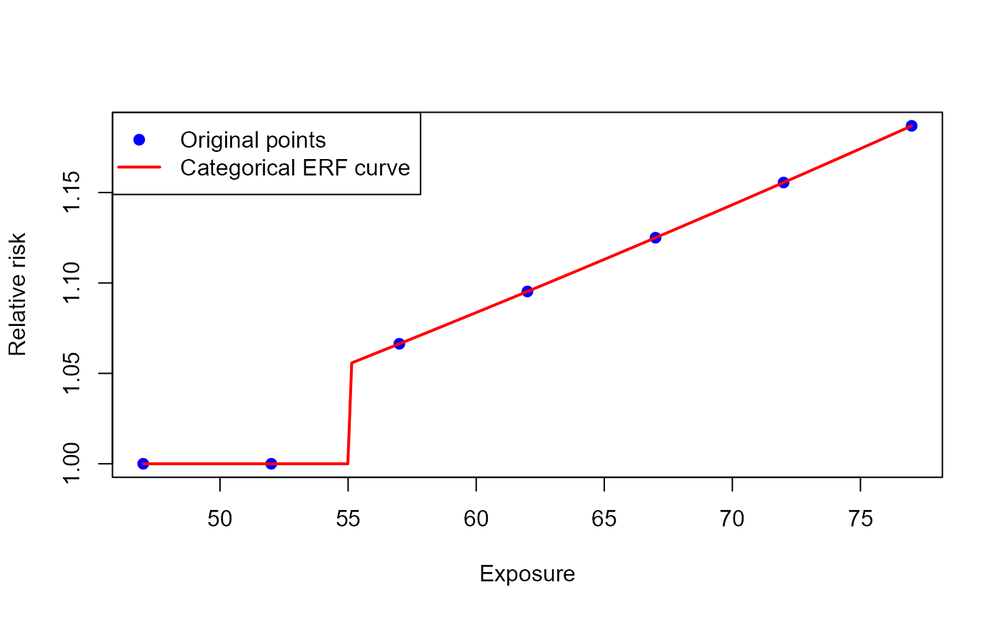
Economic dimension

Monetization

Goal

E.g., to monetize the attributable health impact of a policy that will have health benefits five years from now.

Methodology

In health economic evaluations and economic burden of disease assessments, health impacts may need to be converted into monetary values. For this purpose, you can use monetize().

Several valuation metrics are available, depending on how outcomes are quantified in natural or health units (e.g. cases reduced, deaths prevented, reductions in mortality risk, life-years gained, QALYs gained, DALYs averted). Common metrics include the Value of a Statistical Life (VSL) (OECD 2025) , the Value of a Life-Year (VOLY) (Hammitt 2007) and the Value of a Quality-Adjusted Life-Year (VAQALY) (Bobinac et al. 2010).

Discounting is the practice of converting future costs (or health impacts as previous step to valuating them) into their present value. The underlying rationale is that the value placed on outcomes declines as they occur further in the future. Therefore, future costs and effects are converted into present-value terms to make them comparable over time (Attema, Brouwer, and Claxton 2018).

Discounting is implemented by selecting a discount rate, which is used to compute a discount factor for each time period. This factor is then multiplied by the corresponding future cost (or effect) to express it in present-value terms.

If you need the discounted values of a cost or health outcome, you can call the healthiar function discount(). If you just need the discount factor, you can alternatively call get_discount_factor(). If you just need the inflation factor, you can get_inflation_factor().

Different functional forms can be used to apply discounting. The most common is exponential discounting, also referred to as constant discounting, since outcomes are discounted proportionally as time increases. An alternative is hyperbolic discounting, which tends to better capture human behavior by discounting the near present more heavily than outcomes further in the future (Lipman and Attema 2024)

See below the equations that are used behind these functions.

Inflation factor (without discounting)

As suggested by (Brealey et al. 2023; Samuelson 1937)

$inflation\_factor = (1 + inflation\_rate)^{n\_years}$

Discount factors (without inflation)

Exponential discounting (no inflation)

As suggested by Frederick, Loewenstein, and O’Donoghue (2002)

$discount\_factor = \frac{1}{(1 + discount\_rate)^{n\_years}}$

Hyperbolic discounting Harvey (no inflation)

As suggested by Harvey (1986)

$discount\_factor = \frac{1}{(1 + n\_years)^{discount\_rate}}$

Hyperbolic discounting Mazur (no inflation)

As suggested by Mazur (1987)

$discount\_factor = \frac{1}{1 + (discount\_rate \times n\_years)}$

Discount factors with inflation

Exponential discounting (with inflation) $discount\_and\_inflation\_factor = \frac{1}{((1 + discount\_rate) \times (1 + inflation\_rate))^{n\_years}}$

Hyperbolic discounting Harvey (with inflation) $discount\_and\_inflation\_factor = \frac{1}{(1 + n\_years)^{discount\_rate} \times (1 + inflation\_rate)^{n\_years}}$

Hyperbolic discounting Mazur (with inflation) $discount\_and\_inflation\_factor = \frac{1}{(1 + (discount\_rate \times n\_years)) \times (1 + inflation\_rate)^{n\_years}}$

Function call

monetized_pm_copd <- monetize(
    output_attribute = results_pm_copd,
    discount_shape = "exponential",
    discount_rate = 0.03,
    n_years = 5,
    valuation = 50000 # E.g. EURO
)

Main results

The outcome of the monetization is added to the variable entered to the output_attribute argument, which is results_pm_copd in our case.

Two folders are added:

monetization_main contains the central monetization estimate and the corresponding 95% confidence intervals obtained through the specified monetization.
monetization_detailed contains the monetized results for each unique combination of the input variable estimates that were provided to the initial attribute_health() call.

erf_ci	monetized_impact
central	151041153
lower	58358321
upper	236091201

We see that the monetized impact (discounted) is more than 160 million EURO.

Alternatively, you can also monetize (attributable) health impacts from a non-healthiar source.

results <- monetize(
  impact = 1151,
  valuation = 100
)

Cost-benefit analysis

Goal (e.g.)

E.g., to perform an economic evaluation for an intervention by comparing its benefits and costs via Cost-Benefit Analysis (CBA).

Methodology

The CBA is a type of economic evaluation that compares the costs and the benefits of an intervention, considering both measures expressed in monetary terms.

To perform a CBA, you can use the function cba(). This approach requires monetizing benefits so they can be directly compared with costs. Since interventions typically generate costs and benefits over multi-year time horizons, discounting is a common practice to obtain the present value of future costs and benefits. Depending on the reference guidelines, the discount rate can be specified as the same for costs and benefits or different across them. The outputs of a Cost-Benefit Analysis can be expressed as three main indicators (Boardman et al. 2018): - intervention’s net benefit: the difference between monetized benefits and costs - Cost-Benefit Ratio (CBR): monetized benefits divided by costs and - Return on Investment (ROI): return generated per unit of expenditure by relating net benefits to the intervention’s costs.

An intervention is recommended from a Cost-Benefit Analysis perspective, if it yields a positive net benefit or a positive ROI, or equivalently, a CBR greater than one, meaning that the intervention’s monetized benefits exceed its costs. These three outputs are available when running cba() and are calculated considering the following formulas.

Net Benefit $net\_benefit = benefit - cost$

Cost-Benefit Ratio (CBR) $cbr = \frac{benefit}{cost}$

Return on Investment (ROI) $roi = \frac{benefit - cost}{cost} \times 100$

Function call

Let’s imagine we design a policy that would reduce air pollution to 5 $\mu g/m^3$ , which is the concentration specified in the cutoff_central argument in the initial attribute_health() call. So we could avoid all COPD cases attributed to air pollution.

Considering the cost to implement the policy (estimated at 100 million EURO), what would be the monetary net benefit of such a policy? We can find out using the functions healthiar and cba()

cba <- cba(
    output_attribute = results_pm_copd,
    valuation = 50000,
    cost = 100000000,
    discount_shape = "exponential",
    discount_rate_benefit = 0.03,
    discount_rate_cost = 0.03,
    n_years_benefit = 5,
    n_years_cost = 5
)

Main results

The outcome of the CBA is contained in two folders, which are added to the existing assessment:

cba_main contains the central estimate and the corresponding 95% confidence intervals obtained
cba_detailed contains additional intermediate results for both cost and benefit
- benefit contains results by_year and raw results health_raw
- cost contains the costs of the policy at the end of the period specified in the n_years_cost argument

cba$cba_main |>  
  dplyr::select(benefit, cost, net_benefit) |> 
  knitr::kable()

benefit	cost	net_benefit
151041153	86260878	64780274
58358321	86260878	-27902557
236091201	86260878	149830323

We see that the central and upper 95% confidence interval estimates of avoided attributable COPD cases result in a net monetary benefit of the policy, while the lower 95% confidence interval estimate results in a net cost!

Goal

E.g., to estimate the health impact that is theoretically attributable to the difference in degree of deprivation of the population exposed.

Methodology

Taking into account socio-economic indicators, e.g. a multiple deprivation index (Mogin et al. 2025), the differences in attributable health impacts across the study areas can be estimated (Renard et al. 2019; Otavova et al. 2022).

Social inequalities are quantified as the difference between the least deprived areas (the last n-quantile) and

the most deprived areas or
the population overall.

These differences can be

absolute or
relative.

Difference most deprived vs. least deprived

$absolute\_quantile = first - last$ Where:

$absolute\_quantile$ = Absolute difference between quantiles.
$first$ = Average health impacts in most deprived quantile.
$last$ = Average health impacts in least deprived quantile.

$relative\_quantile = \frac{absolute\_quantile}{last}$

Difference overall vs. least deprived

$absolute\_overall = overall - last$ Where:

$absolute\_overall$ = Absolute difference regarding the overall average.
$overall$ = Overall average health impacts in the study area.
$last$ = Average health impacts in least deprived quantile.

If you assume that the least deprived areas are similar to counter-factual cases (no exposure to deprivation), the relative difference regarding the overall average health impact could be interpreted as some kind of relative risk attributable to social inequalities.

Function call

First, quantify health impacts.

 health_impact <- healthiar::attribute_health(
   age_group = exdat_socialize$age_group,
   exp_central = exdat_socialize$pm25_mean,
   cutoff_central = 0,
   rr_central = exdat_socialize$rr,
   erf_shape = "log_linear",
   rr_increment = 10,
   bhd_central = exdat_socialize$mortality,
   population = exdat_socialize$population,
   geo_id_micro = exdat_socialize$geo_unit)

Second, use the function socialize() entering the whole output of attribute_health() in the argument output_attribute.

social_t <- healthiar::socialize(
  output_attribute = health_impact,
  age_group = exdat_socialize$age_group, # They have to be the same in socialize() and in attribute_health()
  ref_prop_pop = exdat_socialize$ref_prop_pop, # Population already provided in output_attribute
  geo_id_micro = exdat_socialize$geo_unit,
  social_indicator = exdat_socialize$score,
  n_quantile = 10,
  increasing_deprivation = TRUE)

Alternatively, you can directly enter the health impact in the socialize() argument impact.

social <- healthiar::socialize(
  impact = health_impact$health_detailed$results_by_age_group$impact,
  age_group = exdat_socialize$age_group, # They have to be the same in socialize() and in attribute_health()
  ref_prop_pop = exdat_socialize$ref_prop_pop,
  geo_id_micro = exdat_socialize$geo_unit,
  social_indicator = exdat_socialize$score,
  population = exdat_socialize$population, # Population has to be provided because no output_attribute
  n_quantile = 10,
  increasing_deprivation = TRUE)

Main results

#> # A tibble: 4 × 5
#>   parameter      difference_type difference_compared_…¹ difference_value comment
#>   <chr>          <chr>           <chr>                             <dbl> <chr>  
#> 1 impact_rate_s… absolute        last_quantile                   11.5    NA     
#> 2 impact_rate_s… relative        last_quantile                    0.193  NA     
#> 3 impact_rate_s… absolute        overall                         -0.834  It can…
#> 4 impact_rate_s… relative        overall                         -0.0143 It can…
#> # ℹ abbreviated name: ¹difference_compared_with

Multiple deprivation index

Goal

E.g., to estimate the multiple deprivation index (MDI) to use it for the argument social_indicator in the function socialize().

Methodology

Socio-economic indicators (e.g., education level, employment status and family structure) can be condensed into a multiple deprivation index (MDI) (Mogin et al. 2025). For this purpose, the indicators can be normalized using min-max scaling.

The reliability of the MDI can be assessed using Cronbach’s alpha (Cronbach 1951).

$\alpha = \frac{k}{k - 1} \left( 1 - \frac{\sum_{i=1}^{k} \sigma^2_{y_i}}{\sigma^2_x} \right)$ where:

$k$ is the number of items/variables.
$\sigma^2_{y_i}$ is the variance of the $i$ -th item.
$\sum_{i=1}^{k} \sigma^2_{y_i}$ is the sum of the variances of all items.
$\sigma^2_x$ is the total variance of the observed total scores (the sum of all items).

To apply this approach, you should ensure that the data set is as complete as possible. Otherwise, you can try to impute missing data using: - Time-Based Imputation: Linear regression based on historical trends if prior years’ data is complete. - Indicator-Based Imputation: Multiple linear regression if the missing indicator correlates strongly with others.

Imputation models should have an R^2 greater than or equal to 0.7. If R^2 lower than 0.7, consider alternative data sources or methods.

Function call

mdi <- prepare_mdi(
  geo_id_micro = exdat_prepare_mdi$id,
  edu = exdat_prepare_mdi$edu,
  unemployed = exdat_prepare_mdi$unemployed,
  single_parent = exdat_prepare_mdi$single_parent,
  pop_change = exdat_prepare_mdi$pop_change,
  no_heating = exdat_prepare_mdi$no_heating,
  n_quantile = 10,
  verbose = FALSE
)

Note: verbose = FALSE suppresses any output to the console (default: verbose = TRUE, i.e. with printing turned on).

Main results

Function output includes:

mdi_main, a tibble containing the BEST-COST MDI

mdi$mdi_main |> 
  select(geo_id_micro, MDI, MDI_index)

geo_id_micro	MDI	MDI_index
11001	0.2117721	1
11002	0.4319924	8
11004	0.1847750	1
11005	0.3787937	7
11007	0.3121354	5
11008	0.2565185	2
11009	0.2245822	1
11013	0.2140148	1
11016	0.2656597	3
11018	0.3566141	6

The function assesses the reliability of the MDI based on the Cronbach’s alpha value as follows: - 0.9 and higher: Excellent reliability - between 0.8 (included) and 0.9: Good reliability - between 0.7 (included) and 0.8: Acceptable reliability - between 0.6 (included) and 0.7: Questionable reliability - lower than 0.6: Poor reliability

Detailed results

mdi_detailed
- DESCRIPTIVE STATISTICS
- PEARSON’S CORRELATION COEFFICIENTS
- CRONBACH’S α, including the reliability rating this value indicates
- Code for boxplots of the single indicators
- Code for histogram of the MDI’s for the geo units with a normal distribution curve

To reproduce the boxlots run

eval(mdi$mdi_detailed$boxplot)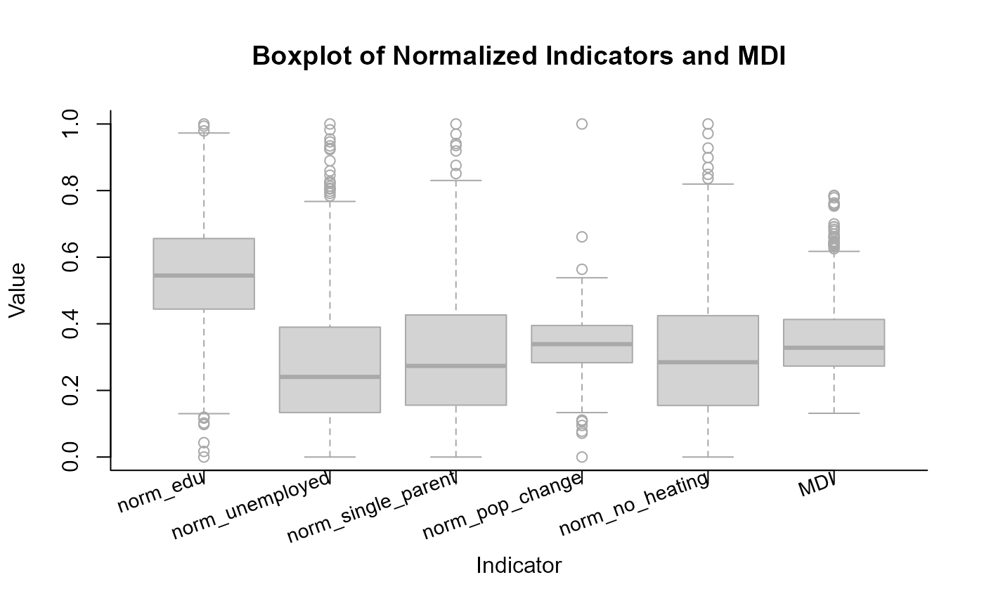

Boxplot of Normalized Indicators and MDI Analogeously, to reproduce the histogram run

eval(mdi$mdi_detailed$histogram)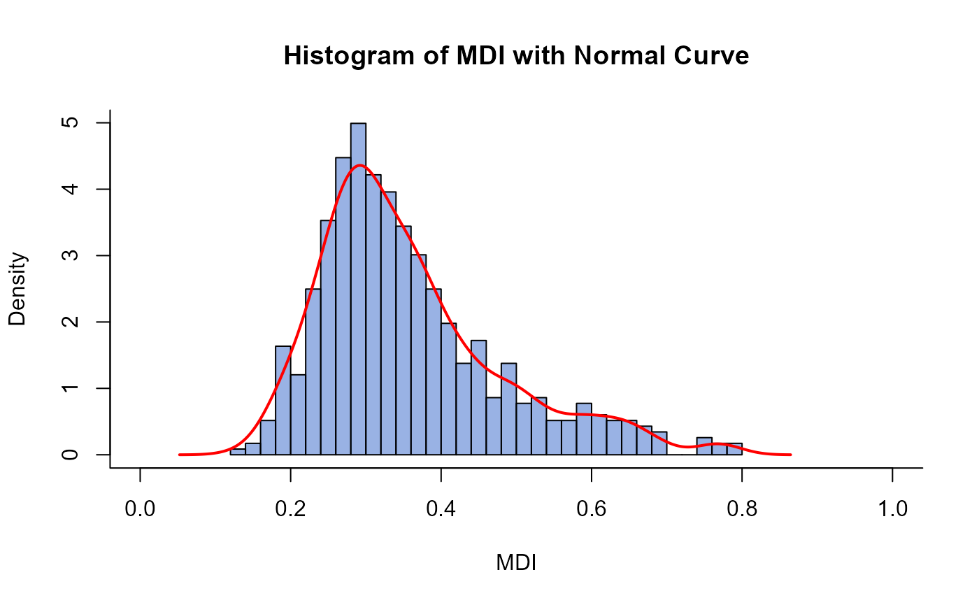

Histogram of MDI with normal curve

Inside pipes

Pipe |>

healthiar can be used inside the native pipes |>. See the example below.

exdat_noise |>
  (\(df) {
    healthiar::attribute_health(
      approach_risk = df$risk_estimate_type,
      exp_central = df$exposure_mean,
      pop_exp = df$exposed,
      erf_eq_central = df$erf
      )$health_main$impact_rounded
    })()

Shorter making used of the base R function with().

exdat_noise |>
      (\(df) {
        with(df, healthiar::attribute_health(
         approach_risk = risk_estimate_type,
         exp_central = exposure_mean,
         pop_exp = exposed,
         erf_eq_central = erf
         ))$health_main$impact_rounded
        })()
#> [1] 348464

Pipe %>%

healthiar can also be used inside magrittr pipes %>% as follows.

exdat_noise %>%
  {
    healthiar::attribute_health(
      approach_risk = .$risk_estimate_type,
      exp_central = .$exposure_mean,
      pop_exp = .$exposed,
      erf_eq_central = .$erf
    )$health_main$impact_rounded
  }

Export and visualize

Exporting and visualizing results is out of scope of healthiar. To export and visualize, you can make use of existing functions in other packages beyond healthiar as indicated below.

Export results

Export as .csv file

Save as .Rdata file

Export to Excel (as .xlsx file)

Visualize results

Visualization is out of scope of healthiar. You can visualize in:

R using base programming or packages such as ggplot2 (Wickham 2016),
Excel (export results first) or
Other tools.

Abbreviations

BHD/bhd = baseline health data

CI = confidence interval

CBA/cba = cost-benefit analysis

exp = exposure

ERF = exposure-response function

RR/rr = relative risk

WHO = World Health Organization

YLL/yll = years of life lost

References

Ahmad, Omar B, Cynthia Boschi Pinto, Alan D Lopez, Christopher JL Murray, Rafael Lozano, and Mie Inoue. 2001. “Age Standardization of Rates: A New WHO Standard.” GPE Discussion Paper Series: No. 31. Geneva: World Health Organization.

Askari, Maryam, and Seyedeh Mahdieh Namayandeh. 2020. “The Difference Between the Population Attributable Risk (PAR) and the Potentioal Impact Fraction (PIF).” Iranian Journal of Public Health 49 (10): 2018–19. https://doi.org/10.18502/ijph.v49i10.4713.

Attema, Arthur E., Werner B. F. Brouwer, and Karl Claxton. 2018. “Discounting in Economic Evaluations.” PharmacoEconomics 36 (7): 745–58. https://doi.org/10.1007/s40273-018-0672-z.

Boardman, Anthony E., David H. Greenberg, Aidan R. Vining, and David L. Weimer. 2018. Cost-Benefit Analysis: Concepts and Practice. 5th ed. Cambridge, UK: Cambridge University Press.

Bobinac, N., J. van Exel, F. F. H. Rutten, and W. B. F. Brouwer. 2010. “Willingness to Pay for a Quality-Adjusted Life-Year: The Individual Perspective.” Value in Health 13 (8): 1046–55. https://doi.org/10.1111/j.1524-4733.2010.00783.x.

Brealey, Richard A., Stewart C. Myers, Franklin Allen, Simon Benninga, and Julian Read. 2023. Principles of Corporate Finance. 14th ed. New York, NY: McGraw-Hill Education.

Cronbach, Lee J. 1951. “Coefficient Alpha and the Internal Structure of Tests.” Psychometrika 16 (3): 297–334. https://doi.org/10.1007/BF02310555.

Devleesschauwer, Brecht, Paul Torgerson, Johannes Charlier, Bruno Levecke, Nicolas Praet, Sophie Roelandt, Suzanne Smit, Pierre Dorny, Dirk Berkvens, and Niko Speybroeck. 2022. Prevalence: Tools for Prevalence Assessment Studies. https://cran.r-project.org/package=prevalence.

Frederick, Shane, George Loewenstein, and Ted O’Donoghue. 2002. “Time Discounting and Time Preference: A Critical Review.” Journal of Economic Literature 40 (2): 351–401. https://doi.org/10.1257/002205102320161311.

GBD 2019 Demographics Collaborators. 2020. “Global Age-Sex-Specific Fertility, Mortality, Healthy Life Expectancy (HALE), and Population Estimates in 204 Countries and Territories, 1950-2019: A Comprehensive Demographic Analysis for the Global Burden of Disease Study 2019.” The Lancet 396 (10258): 1160–1203. https://doi.org/10.1016/S0140-6736(20)30977-6.

GBD 2019 Risk Factors Collaborators. 2020. “Global Burden of 87 Risk Factors in 204 Countries and Territories, 1990–2019.” The Lancet. https://doi.org/10.1016/S0140-6736(20)30752-2.

Hammitt, James K. 2007. “Valuing Changes in Mortality Risk: Lives Saved Versus Life Years Saved.” Review of Environmental Economics and Policy 1 (2): 228–40. https://doi.org/10.1093/reep/rem015.

Harvey, Charles M. 1986. “Value Functions for Infinite-Period Planning.” Management Science 32 (9): 1123–39. https://doi.org/10.1287/mnsc.32.9.1123.

Jerrett, Michael, Richard T Burnett, Bernardo S Beckerman, Michelle C Turner, Daniel Krewski, George Thurston, Randall V Martin, et al. 2013. “Spatial Analysis of Air Pollution and Mortality in California.” American Journal of Respiratory and Critical Care Medicine 188 (5): 593–99. https://doi.org/10.1164/rccm.201303-0609OC.

Kim, Young-Eun, Yoon-Sun Jung, Minsu Ock, and Seok-Jun Yoon. 2022. “DALY Estimation Approaches: Understanding and Using the Incidence-Based Approach and the Prevalence-Based Approach.” J. Prev. Med. Public Health 55 (1): 10–18. https://doi.org/10.3961/jpmph.21.597.

Lehtomäki, Heli, Gunn Marit Aasvang, Gerhard Sulo, Bruce R. Denby, Otto Olavi Hänninen, Michael Brauer, Gavin Pereira, Omid Dadras, and Anette Kocbach Bølling. 2025. “Burden of Disease Attributable to PM2.5 at Low Exposure Levels: Impact of Methodological Choices.” Environmental Health 25 (1): 4. https://doi.org/10.1186/s12940-025-01250-y.

Lipman, Stefan A., and Arthur E. Attema. 2024. “A Systematic Review of Unique Methods for Measuring Discount Rates.” Journal of Risk and Uncertainty 69 (2): 145–89. https://doi.org/10.1007/s11166-024-09439-1.

Mazur, James E. 1987. “An Adjusting Procedure for Studying Delayed Reinforcement.” In Quantitative Analyses of Behavior: Volume v. The Effect of Delay and of Intervening Events on Reinforcement Value, edited by Michael L. Commons, James E. Mazur, John A. Nevin, and Howard Rachlin, 55–73. Hillsdale, NJ: Lawrence Erlbaum Associates.

Miller, B G, and J F Hurley. 2003. “Life Table Methods for Quantitative Impact Assessments in Chronic Mortality.” Journal of Epidemiology & Community Health 57 (3): 200–206. https://doi.org/10.1136/jech.57.3.200.

Miller, Brian G. 2010. “Report on Estimation of Mortality Impacts of Particulate Air Pollution in London.” Institute of Occupational Medicine (IOM). https://cleanair.london/app/uploads/CAL-098-Mayors-health-study-report-June-2010-1.pdf.

Mogin, Gaëlle, Vanessa Gorasso, Jane Idavain, Maria Lepnurm, Sabrina Delaunay-Havard, Anette Kocbach Bølling, Jurgen Buekers, Axel Luyten, Brecht Devleesschauwer, and Carl Michael Baravelli. 2025. “A Scoping Review of Multiple Deprivation Indices in Europe.” European Journal of Public Health 35 (6): 1122–28. https://doi.org/10.1093/eurpub/ckaf190.

Murray, Christopher J L, Majid Ezzati, Alan D Lopez, Anthony Rodgers, and Stephen Vander Hoorn. 2003. “Comparative Quantification of Health Risks Conceptual Framework and Methodological Issues.” Popul. Health Metr. 1 (1): 1.

Murray, Christopher JL, Majid Ezzati, Alan D Lopez, Anthony Rodgers, and Stephen Vander Hoorn. 2003. “Comparative Risk Assessment: Conceptual Framework and Design.” Epidemiology 14 (4): 447–58. https://doi.org/10.1186/1478-7954-1-1.

OECD. 2025. Mortality Risk Valuation in Policy Assessment: A Global Meta-Analysis of Value of Statistical Life Studies. Paris: OECD Publishing. https://doi.org/10.1787/76ca89a2-en.

Otavova, Martina, Christel Faes, Catherine Bouland, Eva De Clercq, Bram Vandeninden, Thierry Eggerickx, Jean-Paul Sanderson, Brecht Devleesschauwer, and Bruno Masquelier. 2022. “Inequalities in Mortality Associated with Housing Conditions in Belgium Between 1991 and 2020.” BMC Public Health 22 (1): 2397. https://doi.org/10.1186/s12889-022-14819-w.

Pozzer, A., S. C. Anenberg, S. Dey, A. Haines, J. Lelieveld, and S. Chowdhury. 2023. “Mortality Attributable to Ambient Air Pollution: A Review of Global Estimates.” GeoHealth 7 (1): e2022GH000711. https://doi.org/https://doi.org/10.1029/2022GH000711.

Renard, Françoise, Brecht Devleesschauwer, Niko Speybroeck, and Patrick Deboosere. 2019. “Monitoring Health Inequalities When the Socio-Economic Composition Changes: Are the Slope and Relative Indices of Inequality Appropriate? Results of a Simulation Study.” BMC Public Health 19 (1): 662. https://doi.org/10.1186/s12889-019-6980-1.

Robert, Christian P, and George Casella. 2004. Monte Carlo Statistical Methods. Springer Texts in Statistics. Springer Science & Business Media. https://doi.org/10.1007/978-1-4757-4145-2.

Rubinstein, Reuven Y., and Dirk P. Kroese. 2016. Simulation and the Monte Carlo Method. John Wiley & Sons. https://doi.org/10.1002/9781118631980.

Samuelson, Paul A. 1937. “A Note on Measurement of Utility.” The Review of Economic Studies 4 (2): 155–61. https://doi.org/10.2307/2967612.

Soares, J., A. González Ortiz, A. Gsella, J. Horálek, D. Plass, and S. Kienzler. 2022. “Health Risk Assessment of Air Pollution and the Impact of the New WHO Guidelines (Eionet Report – ETC HE 2022/10).” Eionet Report -- ETC HE 2022/10. European Topic Centre on Human Health; the Environment. https://doi.org/10.5281/zenodo.7405988.

Steenland, Kyle, and Ben Armstrong. 2006. “An Overview of Methods for Calculating the Burden of Disease Due to Specific Risk Factors.” Epidemiology 17 (5): 512–19. https://doi.org/10.1097/01.ede.0000229155.05644.43.

Strak, Maciek, Danny Houthuijs, and Brigit Staatsen. 2024. “D1.2 Report on the Methodology for Assessing the Burden of Correlated Exposures.” EU Project BEST-COST.

VanderWeele, Tyler J. 2019. “Optimal Approximate Conversions of Odds Ratios and Hazard Ratios to Risk Ratios.” Biometrics 76 (3): 746–52. https://doi.org/10.1111/biom.13197.

WHO. 2003. “Introduction and Methods: Assessing the Environmental Burden of Disease at National and Local Levels.” World Health Organization. https://www.who.int/publications/i/item/9241546204.

———. 2011. “Burden of Disease from Environmental Noise: Quantification of Healthy Life Years Lost in Europe.” World Health Organization. https://www.who.int/publications/i/item/burden-of-disease-from-environmental-noise-quantification-of-healthy-life-years-lost-in-europe.

———. 2020. “Health Impact Assessment of Air Pollution: AirQ+ Life Table Manual.” World Health Organization - Regional Office for Europe. https://www.who.int/europe/publications/i/item/WHO-EURO-2020-1559-41310-56212.

WHO Regional Office for Europe. 2014. WHO Expert Meeting: Methods and Tools for Assessing the Health Risks of Air Pollution at Local, National and International Level. Meeting Report; 12-13 May 2014; Bonn, Germany. Copenhagen: WHO Regional Office for Europe. https://iris.who.int/handle/10665/142940.

Wickham, Hadley. 2014. “Tidy Data.” Journal of Statistical Software 59 (10): 1–23. https://doi.org/10.18637/jss.v059.i10.

———. 2016. Ggplot2: Elegant Graphics for Data Analysis. Springer-Verlag New York. https://ggplot2.tidyverse.org.

About healthiar

Input & output data

Input

Hard coded vs. columns

Hard coded

Columns

Tidy data

Output

Structure

Access

Function examples

Relative risk

Goal

Methodology

Population attributable fraction

Simplified for categorical exposure distribution

Simplified for single exposure value

Function call

Main results

Absolute risk

Goal

Methodology

Function call

Main results

Results per noise exposure band

One exposure category

Multiple geographic units

using relative risk

Goal

Function call

Main results

Detailed results

using absolute risk

Goal

Function call

Main results

Detailed results

Uncertainty

Confidence interval

Goal

Function call

Detailed results

Monte Carlo simulation

Goal

Methodology

General concepts

Distributions used for simulation

Function call

Main results

Detailed results

User-defined ERF

Goal

Function call

Sub-group analysis

by age group

Goal

Function call

Results by age group

by sex

Goal

Function call

Results by sex

by other sub-groups

Goal

Function call

Results by other sub-group

by age, sex and other sub-groups

Goal

Function call

Results by all sub-groups

YLL & deaths with life table

YLL

Goal

Methodology

Data preparation

General concept

Determination of populations in the (first) year of analysis

Entry population

Survival probabilities

About `healthiar`