vivaxmodelr.Rmdtitle: “VivaxModelR: simple version” subtitle: “An R package to simulate P. vivax dynamics” author: “Clara Champagne, Maximilian Gerhards, Justin Lana, Bernardo García Espinosa, Christina Bradley, Óscar González, Justin Cohen, Arnaud Le Menach, Michael White, Emilie Pothin” output: rmarkdown::html_vignette bibliography: bibliography.json vignette: > % % % —
This package contains functions to simulate a compartmental model for Plasmodium Vivax and calculate the associated reproduction number for a given epidemiological setting, based on data on reported local and imported cases. The model includes case management and vector control.
It is based on (white2016?), and can be represented by the following diagram: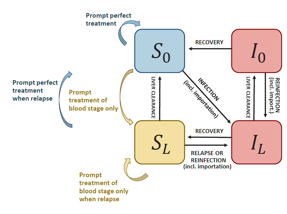
Schematic representation of the model
where \(I_L\) is the proportion of individuals with both blood and liver stage parasites, \(I_0\) is the proportion of individuals with blood stage parasites only, \(S_L\) is the proportion of individuals with liver stage parasites only, and \(S_0\) is the proportion of susceptible individuals.
As in (white2016?), it requires 4 biological parameters: \(\lambda\) (transmission rate, called “lambda” in the package), \(r\) (blood parasites clearance rate), \(\gamma_L\) (liver parasites clearance rate, called “gamma”) and \(f\) (relapse frequency). Values from the literature can be found for \(r\), \(\gamma_L\) and \(f\). The parameter \(\lambda\) is highly setting specific and can be calculated based on incidence and importation data using the functions from this package. This also provides estimates of setting specific reproduction numbers: \(R_0\) (in the absence of control intervention) and \(R_c\) (considering current control interventions).
For more information, please refer to the associated paper ((champagne2022?)).
How to use the package
Calculate the reproduction numbers from data on reported cases
Creating a dummy dataset with reported incidence and the proportion of imported cases (the user should include their real data). Incidence is in cases per 1000 person-year. Each line corresponds to an administrative area or a year of data.
mydata=data.frame(id=c("regionA","regionB"),incidence=c(23,112),prop_import=c(0,0.1))Convert incidence to cases per person day:
mydata$h=incidence_year2day(mydata$incidence)Indicate model intervention parameter values for current case management (\(\alpha\) and \(\beta\)) and vector control (\(\omega\)), as well as the observation rate (\(\rho\)).
The parameter \(\alpha\) (called “alpha” in the package) represents the probability to receive effective cure for the blood stage infection and the parameter \(\beta\) (called “beta”) represents the probability that individuals clear their liver stage infection when receiving their treatment. The parameter \(\omega\) (called “omega”) quantifies the intensity of vector control (0 indicating perfect vector control and 1 indicating the absence of vector control). The observation rate \(\rho\) (called “rho”) indicates the proportion of all infections that are effectively observed and reported in the incidence data. The parameter \(\alpha\) should reflect the proportion of individual effectively cured (for example because they present symptoms, seek care, and receive and adhere to an effective treatment, as in (galactionova2015?) for example).
mydata$alpha=c(0.17, 0.12) # proportion of treated cases
mydata$beta=c(0.43,0.42) # proportion of radical cure
mydata$rho=c(0.18, 0.13) # reporting rate (here, we assume that all treated cases are reported)
mydata$omega=c(1,1)  # no vector control
Run the model and save the results in a new database.
mydata_withR0RC=calibrate_vivax_equilibrium(df=mydata, f=1/72, gamma=1/223, r=1/60, return.all = TRUE)
#> Warning in calibrate_vivax_equilibrium(df = mydata, f = 1/72, gamma = 1/223, :
#> no rho2 parameter, assumed rho2=1
#> Warning in solve_lambda_vivax(h = my.h, r = r, gamma = gamma, f = f, alpha =
#> my.alpha, : imaginary parts discarded in coercion
Visualise the output: several additional columns were created, including \(R_0\) and \(R_c\) for each region/year.
mydata_withR0RC
#>        id incidence prop_import            h alpha beta  rho omega rho2
#> 1 regionA        23         0.0 0.0000630137  0.17 0.43 0.18     1    1
#> 2 regionB       112         0.1 0.0003068493  0.12 0.42 0.13     1    1
#>        lambda        Rc       R0       delta          I
#> 1 0.008913383 1.0266852 1.322669 0.000000000 0.01743379
#> 2 0.007613010 0.9498208 1.129705 0.000269643 0.12462803
The transmission rate lambda has been calibrated to the incidence and import proportion and it can be used to simulate future scenarios. The quantity \(\delta\) (called “delta”) representing the daily importation rate was also calculated based on the observed data.
Simulate a future scenario with the fitted model.
In this section, we will see how to use the calibrated model to simulate the impact of a future intervention, starting from the model equilibrium.
As a first step, the intervention variables describing the new intervention scenario need to be defined. For each intervention, we create an intervention object containing new parameter values after the intervention. For example, we want to increase the proportion of radical cure \(\beta\) from 0.4 to 0.6 (intervention A) or 0.8 (intervention B).
intervention_object0=list(intervention_name="baseline", "alpha.new"=NA, "beta.new"=NA, "omega.new"=NA, "rho.new"=NA )
intervention_objectA=list(intervention_name="intervA", "alpha.new"=NA, "beta.new"=0.6, "omega.new"=NA, "rho.new"=NA )
intervention_objectB=list(intervention_name="intervB", "alpha.new"=NA, "beta.new"=0.8, "omega.new"=NA , "rho.new"=NA)
Now, we use the previously calibrated model (using the values contained in mydata_withR0RC) to simulate the interventions. Make sure that the data frame contains a variable called “id” that identifies uniquely each row.
Now, we simulate the model with the new parameterisation.
my_intervention_list=list(intervention_object0, intervention_objectA, intervention_objectB)
simulation_model= simulate_vivax_interventions(df=mydata_withR0RC, my_intervention_list)
#> Starting from equilibrium
#> simulating from equilibrium
head(simulation_model)
#>        id time         Il          I0         Sl       S0     h        hr    hl
#> 1 regionA    0 0.01376454 0.003669252 0.01421216 0.968354 0.023 0.0129686 0.023
#> 2 regionA  365 0.01376454 0.003669252 0.01421216 0.968354 0.023 0.0129686 0.023
#> 3 regionA  730 0.01376454 0.003669252 0.01421216 0.968354 0.023 0.0129686 0.023
#> 4 regionA 1095 0.01376454 0.003669252 0.01421216 0.968354 0.023 0.0129686 0.023
#> 5 regionA 1460 0.01376454 0.003669252 0.01421216 0.968354 0.023 0.0129686 0.023
#> 6 regionA 1825 0.01376454 0.003669252 0.01421216 0.968354 0.023 0.0129686 0.023
#>          hh       hhl          I p incidence intervention step
#> 1 0.1277778 0.1277778 0.01743379 0        23     baseline    1
#> 2 0.1277778 0.1277778 0.01743379 0        23     baseline    1
#> 3 0.1277778 0.1277778 0.01743379 0        23     baseline    1
#> 4 0.1277778 0.1277778 0.01743379 0        23     baseline    1
#> 5 0.1277778 0.1277778 0.01743379 0        23     baseline    1
#> 6 0.1277778 0.1277778 0.01743379 0        23     baseline    1
The variable time indicates the number of days since baseline. The other variables are the state variables of the model. The variable \(I\) indicates the proportion of all individuals with blood stage infection (\(I=I_L+I_0\)), i.e. prevalence (including any parasite concentration). The variable incidence indicates the incidence per 1000 person year. All variables are detailed in the following table:
| Column name | Description | Unit |
|---|---|---|
| id | Unique identifier of the area | |
| time | Number of days since baseline | days |
| Il | \(I_L\), proportion of individuals with both blood and liver stage parasites | dimensionless |
| I0 | \(I_0\), proportion of individuals with blood stage parasites only | dimensionless |
| Sl | \(S_L\), proportion of individuals with liver stage parasites only | dimensionless |
| S0 | \(S_0\), proportion of susceptible individuals | dimensionless |
| h | Reported incidence | cases per person year if year=T or per person day if year=F |
| hr | Reported incidence due to relapses | cases per person year if year=T or per person day if year=F |
| hl | Local reported incidence | cases per person year if year=T or per person day if year=F |
| hh | Total incidence | cases per person year if year=T or per person day if year=F |
| hhl | Total local incidence | cases per person year if year=T or per person day if year=F |
| I | Prevalence (\(I_L+I_0\)) | dimensionless |
| p | Proportion of imported cases | dimensionless |
| incidence | Reported incidence | cases per 1000 person year |
| intervention | Name of the intervention | |
| step | Simulation step | 1 corresponds to the first simulation from equilibrium |
The model outputs can be represented graphically, for example using the ggplot2 package.
library(ggplot2)
ggplot(simulation_model)+
  geom_line(aes(x=time/365,y=incidence, color=intervention), lwd=1)+
  facet_wrap(id ~., scales = "free_y")+xlab("Year since baseline")
Simulate a future scenario with the fitted model, starting from a previous simulation run
simulation_model_day= simulate_vivax_interventions(df=mydata_withR0RC, my_intervention_list, year=F)
#> Starting from equilibrium
#> simulating from equilibrium
intervention_object0=list(intervention_name="baseline", "alpha.new"=NA, "beta.new"=NA, "omega.new"=NA, "rho.new"=NA )
intervention_objectB2=list(intervention_name="intervB", "alpha.new"=NA, "beta.new"=0.9, "omega.new"=NA, "rho.new"=NA )
my_intervention_list2=list(intervention_object0, intervention_objectA, intervention_objectB2)
simulation_model2= simulate_vivax_interventions(df=mydata_withR0RC, my_intervention_list2, previous_simulation = simulation_model_day, year=F)

ggplot(simulation_model2)+
  geom_line(aes(x=time/365,y=I, color=intervention, linetype=as.factor(step)), lwd=1)+
  facet_wrap(id ~., scales = "free_y")+xlab("Year since baseline")+ylab("Prevalence")
Additional features
Including decay in the vector control parameter
It is possible to include a decay in the vector control parameter \(\omega\). For example, an exponential decay, using the following function:
my_omega=vector_control_exponential_decay(initial_omega = 0.8, half_life = 3, every_x_years = 3, maxtime = 7*365 )
head(my_omega)
#>   time     value
#> 1    0 0.8000000
#> 2    1 0.8001266
#> 3    2 0.8002530
#> 4    3 0.8003794
#> 5    4 0.8005058
#> 6    5 0.8006320
ggplot(my_omega)+  geom_line(aes(x=time/365,y=value), lwd=1)+labs(x="years", y=expression(omega))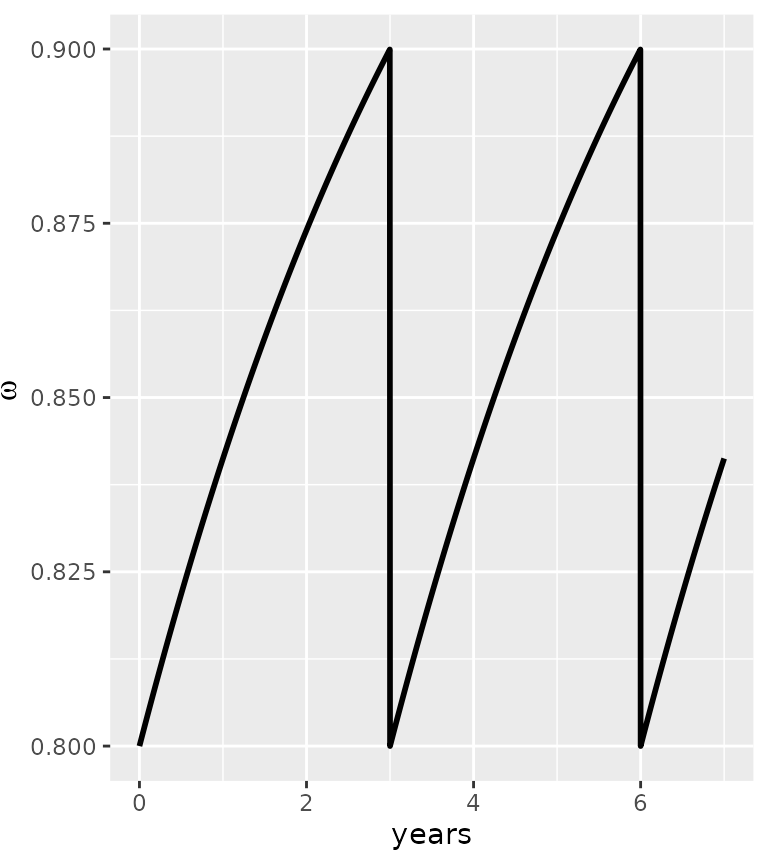
In this example, we implement a vector control intervention every 3 years, with an initial efficacy of \(\omega=0.8\) and a half-life of 3 years. Other patterns can be used, especially derived from the AnophelesModel package (Golumbeanu et al. in prep), as long a the dataset is provided as a dataframe with a “time” and “value” column.
intervention_objectC=list(intervention_name="intervC", "alpha.new"=NA, "beta.new"=NA, "omega.new"=0.8, "rho.new"=NA )
intervention_objectCdecay=list(intervention_name="intervCdecay", "alpha.new"=NA, "beta.new"=NA, "omega.new"=my_omega, "rho.new"=NA )

my_intervention_list_vc=list(intervention_object0, intervention_objectC, intervention_objectCdecay)

simulation_model_vc= simulate_vivax_interventions(df=mydata_withR0RC, my_intervention_list_vc, maxtime = 7*365, year=F)
#> Starting from equilibrium
#> simulating from equilibrium

ggplot(simulation_model_vc)+
  geom_line(aes(x=time/365,y=incidence, color=intervention), lwd=1)+
  facet_wrap(id ~., scales = "free_y")+xlab("Year since baseline")
#> Warning: Removed 1 row containing missing values (`geom_line()`).
Modify the importation rate over time
It is possible to modify the importation parameter \(\delta\) over time. For example, we want to
leave it constant for 1 year, and then make it decrease linearly to zero
over the next 2 years (starting from the initial equilibrium
value).
We write the desired pattern in a dataframe:
my_trend=data.frame(time=c(0, # baseline
                           365, # after 1 year
                           3*365+1 # after 3 years (+1 to ensure the whole 3 year period is entirely covered)
                           ),
                    relative_change=c(1, # initial value is constant (*1)
                                      1, # still constant after 1 year (*1)
                                      0  # equalsto zero after 3 years (*0)
                                      ))
Secondly, we create a database containing all unique regions, their respective value for \(\delta\) and the desired time points:
  full=list()
  full$id=mydata_withR0RC$id # extract all unique regions from previous database
  full$time=c(0,365,3*365+1) # desired time points
  my_delta0=dplyr::left_join(expand.grid( full ), mydata_withR0RC[,c("id","delta")])
#> Joining with `by = join_by(id)`

  my_delta0
#>        id time       delta
#> 1 regionA    0 0.000000000
#> 2 regionB    0 0.000269643
#> 3 regionA  365 0.000000000
#> 4 regionB  365 0.000269643
#> 5 regionA 1096 0.000000000
#> 6 regionB 1096 0.000269643
We now merge this table with the pre-defined trend and build the input database for the package:
my_delta=my_delta0 %>% # create a data.frame with the
    dplyr::left_join(my_trend) %>%
    dplyr::mutate(value=relative_change*delta) %>%
    dplyr::select(id,time,value)
#> Joining with `by = join_by(time)`

my_delta
#>        id time       value
#> 1 regionA    0 0.000000000
#> 2 regionB    0 0.000269643
#> 3 regionA  365 0.000000000
#> 4 regionB  365 0.000269643
#> 5 regionA 1096 0.000000000
#> 6 regionB 1096 0.000000000
This data.frame can then be used in the creation of the intervention object. Other patterns can be used, as long a the dataset is provided as a ata.frame with an “id”, “time” and “value” column.
intervention_objectD=list(intervention_name="baseline", "alpha.new"=NA, "beta.new"=NA, "omega.new"=NA, "rho.new"=NA)
intervention_objectD_delta=list(intervention_name="A", "alpha.new"=NA, "beta.new"=NA, "omega.new"=NA, "rho.new"=NA, "delta.new"=my_delta)

my_intervention_list_delta=list(intervention_objectD,intervention_objectD_delta)

simulation_model_delta=simulate_vivax_interventions(df=mydata_withR0RC, intervention_list = my_intervention_list_delta, year=F, maxtime = 365*3)
#> Starting from equilibrium
#> simulating from equilibrium

ggplot(simulation_model_delta)+
  geom_line(aes(x=time/365,y=incidence, color=intervention), lwd=1)+
  facet_wrap(id ~., scales = "free_y")+xlab("Year since baseline")+ylim(0,NA)
In region A, the importation rate was already equal to zero, therefore, the trajectory remains unchanged.
Including uncertainty quantification in data reporting
Creating a dummy dataset with reported numbers or total cases and local cases, i.e. as opposed to imported cases, and the population size of the area (the user should include their real data). Each line corresponds to an administrative area or a year of data. We also added the reporting and case management parameters for each setting.
mydata_2=data.frame(id=c("regionA","regionB"),cases=c(114,312),cases_local=c(110,290), population=c(10000,5000))
mydata_2$alpha=c(0.18, 0.13) # proportion of treated cases
mydata_2$beta=c(0.43,0.42) # proportion of radical cure
mydata_2$rho=c(0.17, 0.12) # reporting rate (here, we assume that all treated cases are reported)
mydata_2$omega=c(1,1)  # no vector control
Draw 100 samples of the incidence and proportion of imported cases, given the observed total and local number of cases. The uncertainty modelled here is due to population size: for additional information concerning the model, please refer to the associated publication.
mydata_2u=sample_uncertainty_incidence_import(mydata_2, ndraw = 100)Run the model and save the results in a new database.
This database includes 100 replicates of the \(R_0\) and \(R_c\) calculation, including the sampling uncertainty in the incidence and proportion of imported cases, and it can also be used further for simulations.
#nrow(mydata_withR0RC_u)Limitations of the model
The model is a simplified representation of reality, and has therefore some limitations.
Firstly, the model does not include any form of immunity. This simplifcation is acceptable for settings with low to moderate transmission intensity. For high transmission settings (roughly observed annual incidence > 200), other models should be used instead.
Secondly, the model is deterministic and therefore neglects the randomness in very small populations. For very low transmission settings (< 20 reported cases annually), other models should be used instead.
Finally, in some instances, the models cannot provide \(R_0\) and \(R_c\) estimates (NA values, and lambda=-2). This means that the combination of incidence, importation and parameter values does not correspond to any mathematical solution. In this case, please revise the assumptions used.